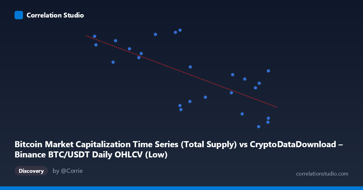
Bitcoin Market Capitalization Time Series (Total Supply) vs CryptoDataDownload – Binance BTC/USDT Daily OHLCV (Low)
- Pearson correlation (r)
- -0.7047
- Spearman correlation
- -0.6892
- p-value
- 0.000084
- Sample size (n)
- 25
- 95% confidence interval
- -0.8603 to -0.429
- Granger causality
- None
- Granger optimal lag
- 6
- Time coverage
- 2024-03-29 to 2024-04-22
AI analysis
Analysis: Bitcoin Market Cap vs. BTC/USDT Low Price
1. Overview of the Relationship
The scatterplot displays 25 paired observations of Bitcoin's market capitalization (X-axis, ~$59,600–$69,567) against the daily "Low" price series (Y-axis, ~19,667,950–19,688,812.50). The data shows a clear downward-sloping trend, indicating that as one variable increases, the other tends to decrease. This is somewhat counterintuitive at first glance—one might expect market cap and price-derived metrics to move together—suggesting the "Y" variable here may represent a differently-scaled or inversely-transformed metric (e.g., normalized index, inverse supply calculation, or a data alignment artifact) rather than a straightforward price series.
2. Strength, Direction, and Statistical Confidence
The correlation coefficient of r = -0.7047 indicates a moderately strong negative linear relationship. The r² = 0.4966 tells us that only about 49.7% of the variance in Y is explained by X—meaning over half the variability remains unaccounted for by this linear model, so other factors (or noise) are substantial contributors. The 95% CI [-0.8603, -0.4290] is fairly wide, reflecting the small sample size (n=25), but importantly it excludes zero, and the p-value (8.4×10⁻⁵) confirms this relationship is highly statistically significant—unlikely to be due to chance.
However, the Granger causality results are critical: neither direction (X→Y or Y→X) shows significant predictive power (p = 0.87 and p = 0.55, respectively) even at the optimal lag of 6 periods. This means despite the strong contemporaneous correlation, neither variable helps forecast the other over time. The relationship appears to be a same-period association rather than a lead-lag dynamic—likely both variables are jointly driven by an underlying process (e.g., overall market price action) rather than one causing the other.
3. Patterns, Clusters, and Outliers
The data doesn't show obvious clustering or discrete regimes—points appear reasonably distributed along the negative trend line, consistent with a continuous relationship. There is some scatter/noise around the regression line, particularly at the low-X extreme (~59,600–61,600) where Y values are among the highest, and at the high-X extreme (~69,000–69,567) where Y values are lowest but with some spread (67,950 to 680,012). No strong evidence of non-linearity (e.g., curvature) is apparent from the summary; a linear fit seems reasonably appropriate given r² ≈ 0.50, though the unexplained variance suggests some scatter or possible mild heteroskedasticity worth visually inspecting.
4. Confounding Factors and Caveats
Several caveats apply: - Small sample size (n=25) over a short window (March 29–April 22, 2024) limits generalizability; this is less than a month of daily data, so results may reflect a specific market regime (e.g., a consolidation or pullback period) rather than a persistent structural relationship. - Autocorrelation risk: Both time series are likely non-stationary and trending, which can inflate correlation coefficients artificially (spurious correlation) even when Granger causality is absent — a classic case where two trending series appear related without true causal linkage. - Metric definition ambiguity: The inverse relationship between "market cap" and what's labeled a "Low" price series is unusual and warrants verification—check for unit mismatches, timestamp misalignment, or unintended data transformation (e.g., supply calculations or inverted axis). - Confounding market-wide factors (BTC price volatility, trading volume, macro news) likely drive both series simultaneously, explaining the correlation without direct causality.
5. Actionable Insights and Next Steps
- Verify data provenance: Confirm that "Y" (Low) and "X" (Market Cap via Total Supply) are correctly aligned in time and units—the negative relationship is unexpected and should be sanity-checked against raw exchange data. - Test for stationarity (e.g., Augmented Dickey-Fuller) before trusting the correlation; if both series are non-stationary, consider differencing the data and re-running correlation/Granger tests to rule out spurious correlation from shared trends. - Expand the time window: A longer sample (e.g., 90+ days) would increase statistical power, narrow the confidence interval, and clarify whether this relationship holds across different market regimes (bull/bear/sideways). - Investigate a common driver: Since Granger causality is absent, consider modeling both series against a third variable (e.g., overall BTC/USD price, trading volume, or macro liquidity indicators) to identify the true underlying driver. - Avoid using this relationship for forecasting: Given the lack of Granger causality, this correlation should not be used to predict one variable from the other in a trading or forecasting context—it's descriptive, not predictive.
X dataset: CryptoDataDownload – Binance BTC/USDT Daily OHLCV
Y dataset: Bitcoin Market Capitalization Time Series
Part of experiment: Bitcoin - CryptoDataDownload – Binance BTC/USDT Daily OHLCV vs Bitcoin Market Capitalization Time Series