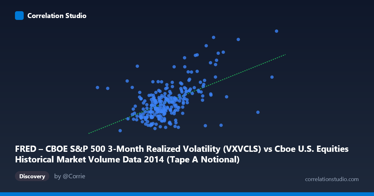
FRED – CBOE S&P 500 3-Month Realized Volatility (VXVCLS) vs Cboe U.S. Equities Historical Market Volume Data 2014 (Tape A Notional)
- Pearson correlation (r)
- 0.552
- Spearman correlation
- 0.4948
- p-value
- 0
- Sample size (n)
- 252
- 95% confidence interval
- 0.4598 to 0.6325
- Granger causality
- None
- Granger optimal lag
- 1
AI analysis
Analysis: CBOE S&P 500 3-Month Realized Volatility vs. Tape A Notional Volume (2014)
Relationship Overview The scatterplot reveals a moderate positive relationship between Cboe U.S. Equities market volume (Tape A Notional) on the X-axis and the CBOE S&P 500 3-Month Realized Volatility index (VXVCLS) on the Y-axis across 252 trading days in 2014. The linear regression equation (y = 6.60×10⁻¹⁰x + 9.95) confirms that as daily notional trading volume increases, realized volatility tends to rise as well — a directionally intuitive result, since elevated market activity is frequently associated with periods of heightened uncertainty or price discovery. The relationship is visible but far from deterministic, with substantial scatter around the regression line throughout the cloud of data points.
Correlation Strength and Statistical Significance The Pearson correlation of r = 0.5520 indicates a moderate positive association, and the R² of 0.3047 means that approximately 30.5% of the variance in realized volatility is explained by notional trading volume — leaving nearly 70% attributable to other factors. The 95% confidence interval of [0.4598, 0.6325] is meaningfully above zero and relatively tight given the sample size (n = 252), and the p-value of effectively zero confirms this correlation is highly statistically significant and unlikely to be a sampling artifact. However, statistical significance should not be conflated with practical predictive power; the moderate R² underscores that volume alone is an incomplete predictor of volatility. Critically, Granger causality tests reveal no significant temporal predictive direction in either direction (X→Y: F = 2.65, p = 0.10; Y→X: F = 0.62, p = 0.43). This means that past volume values do not reliably predict future volatility, and vice versa — the relationship is contemporaneous rather than leading/lagging, substantially limiting its utility for forecasting.
Notable Patterns, Clusters, and Outliers The sample points reveal several noteworthy structural features. The bulk of observations cluster in the X range of roughly 7–10 billion (notional volume) and Y range of 13–17 (volatility), forming a dense core consistent with "normal" 2014 market conditions. However, there are clear high-leverage outliers worth flagging: points near (11.8B, 23.09), (13.6B, 22.85), and (12.3B, 12.87) sit far from the central mass. The first two suggest episodes where both volume and volatility spiked together — likely corresponding to specific market stress events in late 2014 (e.g., the October 2014 equity selloff). The third outlier (12.3B notional, but only 12.87 volatility) is particularly anomalous, suggesting a high-volume day that did not accompany elevated volatility, possibly driven by mechanical or end-of-period volume flows. Additionally, the point at (3.6B, 17.26) represents an unusually low-volume day with above-average volatility — a pattern inconsistent with the general trend and potentially corresponding to a holiday-shortened session or data irregularity.
Confounding Factors and Interpretive Caveats Several important caveats apply. First, directionality and dataset labeling warrant scrutiny: the X-axis is labeled as realized volatility data while drawing from the volume dataset, and vice versa for Y — this axis-label inversion (noted in the metadata) could affect interpretation and should be verified before drawing conclusions. Second, the relationship between volume and volatility is well-documented in market microstructure literature as a joint endogenous response to information arrival rather than a causal chain; both variables react to news simultaneously, which explains the lack of Granger causality. Third, 2014 was a relatively low-volatility year overall with a discrete spike in October, meaning the correlation may be heavily influenced by that cluster of extreme observations — removing them could substantially weaken the measured r. Finally, Tape A (NYSE-listed securities) notional volume is only a partial proxy for overall market activity, and the 3-month realized volatility horizon may dampen responsiveness to short-lived volume spikes.
Actionable Insights and Further Investigation Practitioners should treat volume as a contemporaneous signal of elevated volatility regimes rather than a predictive tool. For trading desks or risk managers, real-time spikes in notional volume may serve as a concurrent indicator warranting volatility reassessment, but not as an advance warning system given the failed Granger tests. For further investigation, it would be valuable to: (1) test non-linear specifications (e.g., log-log regression), as volatility-volume relationships often follow power-law dynamics; (2) segment the analysis by removing the October 2014 stress period to assess whether the correlation is regime-dependent; (3) incorporate VIX (implied volatility) alongside VXVCLS to distinguish realized from expected volatility dynamics; and (4) examine whether intraday volume patterns carry stronger predictive signal than daily aggregates. A regime-switching or quantile regression framework could also reveal whether the volume-volatility relationship strengthens meaningfully in high-stress periods — a finding with direct relevance to risk model calibration.
X dataset: Cboe U.S. Equities Historical Market Volume Data 2014
Y dataset: FRED – CBOE S&P 500 3-Month Realized Volatility
Part of experiment: Daily - Cboe U.S. Equities Historical Market Volume Data 2014 vs FRED – CBOE S&P 500 3-Month Realized Volatility