VIX Volatility Index Daily (FRED) (VIXCLS) vs Cboe U.S. Equities Historical Market Volume Data 2009 (Total Shares)
- Pearson correlation (r)
- 0.5191
- Spearman correlation
- 0.5574
- p-value
- 0
- Sample size (n)
- 252
- 95% confidence interval
- 0.4227 to 0.604
- Granger causality
- None
- Granger optimal lag
- 1
AI analysis
Analysis: VIX Volatility Index vs. Total Shares Traded (2009)
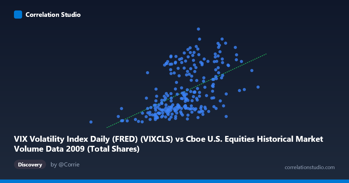
Relationship Overview The scatterplot reveals a moderate positive relationship between the VIX Volatility Index and total shares traded on U.S. equities exchanges throughout 2009. As the VIX rises — indicating higher implied volatility and market fear — trading volume in total shares tends to increase as well. This is broadly consistent with established market microstructure theory: periods of elevated uncertainty drive both institutional hedging activity and retail panic trading, inflating overall share volume. The linear regression equation (y = 3.03×10⁻⁸x + 8.45) reflects this upward trend, though the wide scatter around the regression line immediately signals that the relationship is far from deterministic.
Correlation Strength and Statistical Framing The Pearson correlation of r = 0.519 indicates a moderate positive association, but the r² of 0.2695 is the more sobering figure — only about 27% of the variance in VIX is explained by total share volume, leaving roughly 73% attributable to other forces. The 95% confidence interval of [0.42, 0.60] is meaningfully bounded away from zero, and the p-value of effectively 0 confirms this is not a chance finding at n = 252. However, statistical significance here is partly a function of a large underlying population (N = 3,232), so practical significance deserves separate scrutiny. Critically, Granger causality tests find no significant predictive direction in either direction (X→Y: F = 0.42, p = 0.516; Y→X: F = 1.04, p = 0.308). This means that even though the two variables co-move, neither reliably predicts the other temporally at a one-period lag — ruling out simple lead-lag trading strategies based on this pairing alone.
Notable Patterns, Clusters, and Outliers The sample points reveal several notable structural features. There is a dense central cluster of observations where VIX values between roughly 700M–900M (X) correspond to VIX readings of 20–35, suggesting these represent the calmer mid-year 2009 period as markets began stabilizing post-crisis. A secondary high-volume, high-VIX cluster is visible in the upper-right quadrant (X 950M, Y 40), likely corresponding to early 2009 when residual financial crisis fear kept volatility elevated while deleveraging drove heavy trading. The point (192,269,942, 19.47) stands out as a pronounced low-volume, low-VIX outlier — possibly a holiday-shortened trading session or data anomaly. Several high-VIX readings (45) occur across a wide range of share volumes, hinting at heteroscedasticity: variance in volume appears to fan out at higher VIX levels, which would violate ordinary least squares assumptions and inflate prediction error at the extremes.
Confounding Factors and Caveats Several confounders complicate a causal interpretation. First, 2009 is a structurally unusual year — it encompasses both the tail end of the global financial crisis and a historic market recovery beginning in March, meaning the VIX-volume relationship may be regime-dependent rather than stable. Second, day-of-week and holiday effects artificially suppress volume on certain trading days regardless of volatility. Third, both series may be jointly driven by macro news events (Federal Reserve announcements, earnings seasons, stimulus legislation), making spurious co-movement likely. Fourth, the axis labels appear swapped in the dataset metadata — VIX is listed on the X-axis from the equities volume dataset and vice versa — which warrants a data integrity check before drawing firm conclusions. Finally, the linear model assumes a constant marginal effect of volume on VIX across the entire range, which the heteroscedastic scatter clearly contradicts.
Actionable Insights and Further Investigation Practitioners and researchers should consider several next steps. Regime-segmentation analysis — splitting the data into pre- and post-March 2009 recovery periods — would test whether the correlation is driven primarily by crisis-era observations. Non-linear modeling (e.g., a log-log transformation or spline regression) may better capture the apparent variance expansion at high VIX levels. Given the failed Granger causality result, higher-frequency intraday data might reveal lag structures invisible at the daily level. It would also be valuable to control for known confounders such as S&P 500 returns, macro announcement days, and options expiration dates in a multivariate framework. Finally, replicating this analysis across other years (2008, 2010) would clarify whether the observed r ≈ 0.52 is a stable structural feature of U.S. equity markets or an artifact of the extraordinary volatility environment of 2009.
X dataset: Cboe U.S. Equities Historical Market Volume Data 2009
Y dataset: VIX Volatility Index Daily (FRED)
Part of experiment: Daily - Cboe U.S. Equities Historical Market Volume Data 2009 vs VIX Volatility Index Daily (FRED)