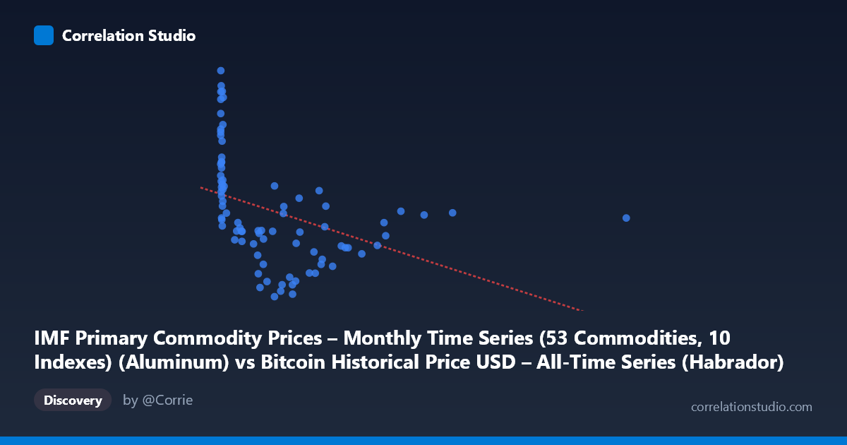
IMF Primary Commodity Prices – Monthly Time Series (53 Commodities, 10 Indexes) (Aluminum) vs Bitcoin Historical Price USD – All-Time Series (Habrador) (Price)
- Pearson correlation (r)
- -0.4008
- Spearman correlation
- -0.661
- p-value
- 0.000174
- Sample size (n)
- 83
- 95% confidence interval
- -0.5674 to -0.2026
- Granger causality
- None
- Granger optimal lag
- 10
- Time coverage
- 2010-08-01 to 2017-06-01
- Recomputed on refreshed data
- 2026-10-24 (r was -0.4008)
AI analysis
Analysis: Aluminum Prices vs. Bitcoin Historical Prices
1. What the Visualization Reveals
The scatterplot shows a weak-to-moderate negative relationship between the aluminum price index (X-axis) and Bitcoin price (Y-axis). The data is heavily clustered at low X-values (aluminum readings near 0–50), with a dense cloud of points showing Bitcoin prices ranging widely (roughly 1,800–2,650) even when aluminum values are nearly identical. As X increases beyond ~600, the point density thins dramatically, with only a handful of high-X observations (997, 1089, 1230, 1402, 2452) trailing off toward the lower end of the Y range (~1,700–1,920). This creates a visual impression of decline, but it's driven largely by a small number of sparse, high-leverage points rather than a consistent trend across the full range.
2. Strength, Direction, and Statistical Uncertainty
The Pearson correlation (r = -0.401) indicates a weak-to-moderate negative linear association, with r² = 0.161 meaning only about 16% of the variance in Bitcoin price is explained by aluminum price — leaving ~84% attributable to other factors. The 95% CI [-0.567, -0.203] is fairly wide and excludes zero, and the p-value (0.000174) confirms this correlation is statistically significant and unlikely due to chance in this sample. However, statistical significance does not imply practical or causal strength — an r² this low means aluminum prices are a poor standalone predictor of Bitcoin price. Critically, the Granger causality tests show no significant predictive relationship in either direction (X→Y: p=0.955; Y→X: p=0.430), meaning neither series helps forecast the other over time. This strongly suggests the correlation is not driven by a genuine lead-lag or causal mechanism, but more likely reflects a spurious relationship — both series may be independently trending over the 2010–2017 window (e.g., Bitcoin's dramatic secular rise) without any real interaction.
3. Notable Patterns and Outliers
The data is extremely right-skewed in X (mean 321 vs. median much lower, stdev 405.64), with over half the observations compressed below X=50. This creates a classic "hook" pattern: a vertical scatter at low X (where Bitcoin varies from 1,470 to 2,667) followed by a sparse tail of high-X points that happen to cluster at moderate Y-values (1,700–1,920). This tail exerts disproportionate leverage on the regression slope — removing just the 5–6 points above X=900 could substantially change or eliminate the negative slope. The note that Spearman ρ exceeds Pearson r reinforces that the relationship may be non-linear or driven by rank-order/monotonic effects rather than a true linear trend, and possibly by these leverage points rather than a smooth curve.
4. Confounding Factors and Caveats
The most important caveat is time confounding: both variables are time series covering 2010–2017, and Bitcoin's price during this period followed a well-documented long-term upward trajectory independent of commodity markets, punctuated by bubbles and crashes (e.g., late 2013, 2017 run-up). Aluminum prices reflect industrial demand, global manufacturing cycles, and macroeconomic conditions largely unrelated to cryptocurrency markets. Any observed correlation is likely a byproduct of shared temporal trends rather than economic linkage — a hallmark of spurious correlation between unrelated time series. Additionally, small sample size (n=83) relative to the full monthly series (N=449) and uneven time sampling (monthly commodity data vs. more granular Bitcoin prices) may introduce alignment/aggregation artifacts. The skewed X distribution further violates assumptions of standard linear correlation, inflating sensitivity to outliers.
5. Recommendations for Further Investigation
Given the lack of Granger causality and low r², this correlation should not be used for predictive or trading purposes. To determine if any genuine relationship exists, analysts should: (1) detrend both series (e.g., using differences or returns rather than levels) to control for shared temporal drift and re-test correlation; (2) examine the relationship after excluding or winsorizing the sparse high-aluminum outliers to check robustness; (3) test non-linear or rank-based models (e.g., Spearman, polynomial fits) given the noted divergence between Spearman and Pearson coefficients; and (4) incorporate additional macro variables (USD index, equity markets, inflation expectations) that may better explain Bitcoin's price action than a single industrial commodity. Absent stronger causal or mechanistic justification, this pairing is best treated as illustrative of spurious correlation risk in time-series analysis rather than a meaningful economic relationship.
X dataset: Bitcoin Historical Price USD – All-Time Series (Habrador)
Y dataset: IMF Primary Commodity Prices – Monthly Time Series (53 Commodities, 10 Indexes)
Part of experiment: Bitcoin - Bitcoin Historical Price USD – All-Time Series (Habrador) vs IMF Primary Commodity Prices – Monthly Time Series (53 Commodities, 10 Indexes)