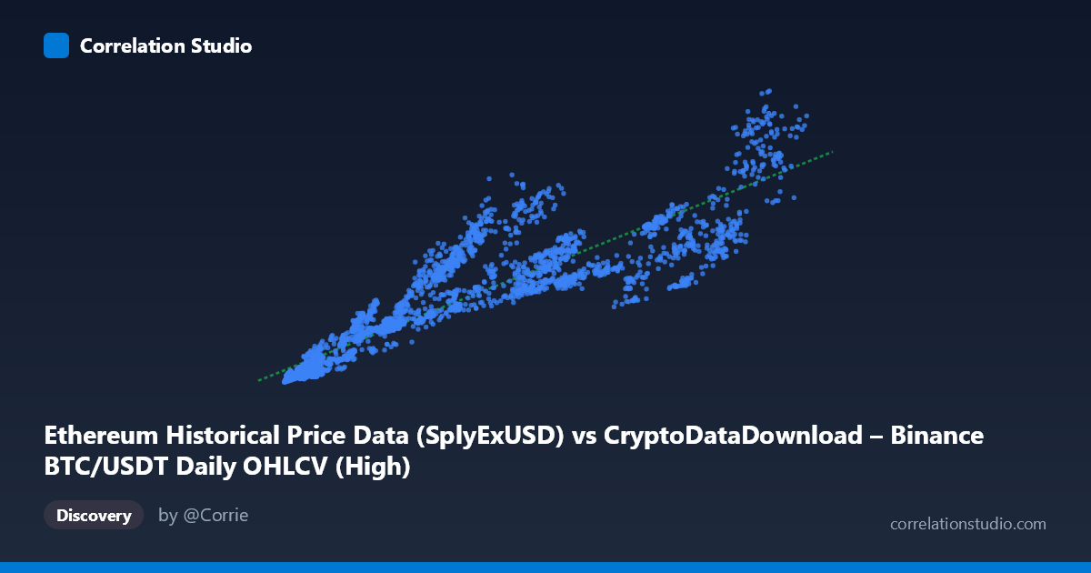
Ethereum Historical Price Data (SplyExUSD) vs CryptoDataDownload – Binance BTC/USDT Daily OHLCV (High)
- Pearson correlation (r)
- 0.9064
- Spearman correlation
- 0.9442
- p-value
- 0
- Sample size (n)
- 3191
- 95% confidence interval
- 0.9 to 0.9124
- Granger causality
- None
- Granger optimal lag
- 10
AI analysis
Analysis of the X–Y Relationship
1. Overview of the Relationship
The scatterplot depicts a strong positive association between the X variable (labeled as Ethereum's SplyExUSD but sourced from a BTC/USDT OHLCV dataset — see caveats below) and Y (Binance BTC/USDT daily high price). As X increases from roughly 3,300 to 126,000, Y rises correspondingly from ~1.4B to ~95.6B, tracing a broadly linear upward trend. The sampled data points confirm this pattern consistently: low-X observations (e.g., X≈4,000–10,000) cluster near Y≈2.4B–7.7B, while high-X observations (X≈100,000–111,000) correspond to Y≈53B–95B. The fitted linear model (y = 548,305x + 3.42B) captures this trend reasonably well.
2. Strength, Direction, and Statistical Confidence
The Pearson correlation of r = 0.9064 indicates a strong positive linear relationship, with r² = 0.8215 meaning approximately 82% of the variance in Y is statistically explained by X — a substantial but not complete fit, leaving ~18% of variance attributable to other factors or nonlinearity. The 95% confidence interval [0.900, 0.912] is tight, and the p-value of 0 (effectively <0.0001) confirms this correlation is highly unlikely to be due to chance, especially given the large sample (n=3,191). However, the Granger causality tests reveal an important caveat: neither direction (X→Y or Y→X) shows significant predictive causality at the optimal lag of 10 periods (p=0.886 and p=0.834, respectively). This means that despite the strong contemporaneous correlation, X does not help forecast future values of Y (or vice versa) beyond what Y's own history provides — the relationship appears to be a co-movement or shared-driver phenomenon rather than one variable temporally leading the other.
3. Notable Patterns and Features
The data shows some heteroskedasticity — variance in Y appears to increase at higher X values (e.g., at X≈84,000, Y ranges from 27.4B to 38.2B across different samples), suggesting the relationship may not be perfectly linear or homoscedastic. There are also mild signs of curvature: at very low X (<10,000), Y values are tightly clustered near the regression line, but scatter widens considerably in the mid-to-upper X range (60,000–90,000), where Y estimates diverge by as much as 10-15B for similar X values. This fanning pattern could indicate a multiplicative or exponential component to the true relationship, or the presence of an unobserved third variable (like market volatility or trading volume) modulating the strength of the linear link at higher price levels.
4. Confounding Factors and Caveats
A critical concern is the data provenance: both axes reference "Binance BTC/USDT Daily OHLCV" — the X-axis label mentions Ethereum's SplyExUSD but the described dataset is BTC/USDT OHLCV, and Y is explicitly the BTC/USDT High price. This raises strong suspicion that X and Y are either the same underlying asset measured differently (e.g., a supply metric vs. price) or mislabeled/duplicated data, which would produce spurious high correlation purely due to shared origin rather than genuine economic causality. Additionally, cryptocurrency prices are notoriously non-stationary and trend together due to macro factors (overall market sentiment, USD liquidity, regulatory news) rather than direct causal links between specific metrics. The time coverage (2017–2026) spans multiple bull/bear cycles, during which both variables likely trended upward together simply due to shared temporal drift, which can inflate correlation without indicating a meaningful functional relationship (a classic spurious-correlation risk with non-stationary time series).
5. Suggested Next Steps
Before drawing conclusions, verify the data labeling/source discrepancy — confirm whether X truly represents an ETH supply metric or is actually BTC-related data mislabeled. If the relationship is genuine, consider testing for cointegration (rather than simple correlation) given the non-stationary, trending nature of crypto price/supply data, and use differenced or log-transformed series to reduce spurious correlation from shared trends. Investigate the heteroskedastic fan pattern by segmenting the data into low/mid/high X regimes and fitting separate models, or trying a log-log or power-law fit to better capture potential nonlinear scaling. Finally, since Granger causality was insignificant, explore whether a third variable (e.g., overall crypto market cap, BTC dominance, or macro liquidity indices) might jointly drive both series, which would better explain the observed correlation without implying direct causality between X and Y.
X dataset: CryptoDataDownload – Binance BTC/USDT Daily OHLCV
Y dataset: Ethereum Historical Price Data
Part of experiment: Bitcoin - CryptoDataDownload – Binance BTC/USDT Daily OHLCV vs Ethereum Historical Price Data