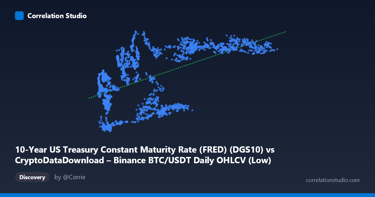
10-Year US Treasury Constant Maturity Rate (FRED) (DGS10) vs CryptoDataDownload – Binance BTC/USDT Daily OHLCV (Low)
- Pearson correlation (r)
- 0.5746
- Spearman correlation
- 0.5471
- p-value
- 0
- Sample size (n)
- 2197
- 95% confidence interval
- 0.5459 to 0.6019
- Granger causality
- None
- Granger optimal lag
- 1
- Time coverage
- 2017-08-17 to 2026-06-25
- Recomputed on refreshed data
- 2026-10-22 (r was 0.5746)
AI analysis
Analysis: BTC Price vs. 10-Year Treasury Yield
Note on axis labeling: The metadata appears reversed — X is described as the 10-Year Treasury rate but ranges from ~2,800 to 123,000 (clearly BTC/USDT price), while Y ranges from 0.52 to 4.98 (clearly the Treasury yield in percent). The analysis below treats X as BTC price and Y as the 10-Year Treasury yield, consistent with the actual data values.
1. What the Visualization Reveals The scatterplot shows a moderate positive association between Bitcoin's price level and the 10-Year Treasury yield over the 2017–2026 sample period. As BTC price rises from the thousands into the tens/hundreds of thousands, the corresponding Treasury yield tends to sit higher on average — rising from roughly 0.5–2% in the low-price regime toward 4–4.7% in the high-price regime. However, the relationship is far from a tight line; at any given BTC price level, yield values are spread across a wide range (e.g., at BTC ≈ 9,000–10,000, yields range from 0.69 to 2.95).
2. Strength, Direction, and Statistical Confidence The correlation coefficient (r = 0.572) indicates a moderate positive relationship, with R² = 0.327 meaning only about 33% of the variance in Treasury yields is explained by BTC price (or vice versa) — leaving roughly two-thirds of the variance driven by other factors. The 95% CI [0.543, 0.600] is fairly tight given the large sample (n=2,183), and the p-value ≈ 0 confirms the correlation is highly statistically significant — this is a real, non-random association, not noise. However, statistical significance with large N should not be conflated with practical predictive strength; R²=0.33 is a modest fit. Critically, the Granger causality tests show no significant predictive direction in either direction (BTC→Yield: p=0.137; Yield→BTC: p=0.603) at lag 1. This means neither series reliably "leads" the other in a short-term forecasting sense — the correlation likely reflects both series responding to a shared macro backdrop (e.g., monetary policy regime, risk appetite, inflation expectations) rather than one directly causing movements in the other.
3. Patterns, Clusters, and Outliers The data shows a clustered, regime-like structure rather than a smooth continuous trend. Low BTC prices (< 20,000) show a bimodal yield spread — some points cluster near low yields (0.7–2.0%) and others near higher yields (3.5–4.3%), suggesting BTC lingered at similar price levels during both the low-rate 2017–2020 period and a subsequent low-price/high-rate period (e.g., 2022 bear market coinciding with Fed hiking cycles). At high BTC prices (60,000), yields consistently cluster in the 4.0–4.7% band with much less dispersion, suggesting a stronger, more homogeneous association in the higher-price regime. This non-linearity/clustering suggests the relationship may be piecewise or driven by distinct market epochs rather than one continuous linear process.
4. Confounding Factors and Caveats This is a classic spurious/co-trending time-series correlation risk: both BTC price and Treasury yields have generally trended upward over 2017–2026 due to unrelated secular forces — BTC's adoption-driven bull markets and the Fed's post-pandemic hiking cycle both happened to rise across overlapping periods. Neither series is stationary, which inflates correlation estimates and violates assumptions of standard r/R² interpretation. Other confounders include: inflation expectations, global liquidity conditions, equity market risk sentiment, and BTC-specific idiosyncratic events (halvings, exchange collapses, regulatory news) that have nothing to do with rates. The lack of Granger causality reinforces that this is likely a coincidental co-trend rather than a causal linkage.
5. Suggestions for Further Investigation To draw more robust conclusions: (1) difference or detrend both series (e.g., use daily returns/changes rather than levels) and re-run correlation and Granger tests to check if the relationship holds after removing shared trend components; (2) test for cointegration (e.g., Engle-Granger or Johansen test) to see if a long-run equilibrium relationship exists despite no short-run Granger causality; (3) segment the analysis by macro regime (zero-rate era vs. hiking cycle) to check if the relationship is regime-dependent rather than stable; (4) include control variables like DXY (dollar index), equity indices (S&P 500), or inflation (CPI) to isolate whether yields matter independently of broader risk-on/risk-off dynamics. Given weak causality, this pair is likely more useful as a macro-context indicator than a direct forecasting input.
X dataset: CryptoDataDownload – Binance BTC/USDT Daily OHLCV
Y dataset: 10-Year US Treasury Constant Maturity Rate (FRED)
Part of experiment: Bitcoin - CryptoDataDownload – Binance BTC/USDT Daily OHLCV vs 10-Year US Treasury Constant Maturity Rate (FRED)