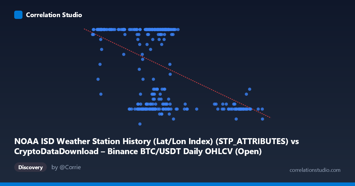
NOAA ISD Weather Station History (Lat/Lon Index) (STP_ATTRIBUTES) vs CryptoDataDownload – Binance BTC/USDT Daily OHLCV (Open)
- Pearson correlation (r)
- -0.4704
- Spearman correlation
- -0.3123
- p-value
- 0
- Sample size (n)
- 355
- 95% confidence interval
- -0.5476 to -0.3851
- Granger causality
- None
- Granger optimal lag
- 1
AI analysis
Analysis of Scatterplot Relationship
1. Overview of the Visualization
The scatterplot displays a moderate negative relationship between the X variable (values ranging ~39,568–106,134) and Y variable (bounded between 5 and 24). Notably, Y appears to behave almost like a discretized or capped variable — a large cluster of points sits at or near the maximum value of 24, while another dense cluster occupies the low end (7–12). This bimodal clustering, rather than a smooth linear cloud, is the dominant visual feature and suggests the relationship is driven more by two distinct regimes than by a continuous linear trend.
2. Strength, Direction, and Statistical Confidence
The correlation coefficient of r = -0.4704 indicates a moderate negative linear association: as X increases, Y tends to decrease. However, r² = 0.2212 shows that only about 22% of the variance in Y is explained by X — meaning nearly 78% of Y's variability is driven by other factors or noise. The 95% confidence interval [-0.5476, -0.3851] is fairly tight and does not cross zero, and the p-value of ~0 confirms the correlation is statistically significant and not due to chance, given the large sample (n=355). That said, statistical significance here reflects sample size more than practical predictive power — r² of 0.22 is a weak-to-moderate effect size in practical terms. Critically, the Granger causality tests show no significant predictive direction in either direction (X→Y: p=0.71; Y→X: p=0.26). This means that despite the contemporaneous correlation, neither variable reliably predicts future values of the other in a time-series sense — the relationship, if causal, is not temporally sequential in the lag structure tested.
3. Patterns, Clusters, and Outliers
The most striking feature is the ceiling effect at Y=24: many points across a wide X range (roughly 42,000–73,000) sit exactly at this maximum, suggesting Y may be capped, saturated, or categorically encoded near this dataset's boundary. Separately, a cluster of low Y values (7–12) appears concentrated in two X sub-ranges: one in the 60,000–70,000 zone and another at higher X values (90,000–100,000). This creates a fan/wedge-like shape rather than a uniform linear scatter — variance in Y is much higher at moderate X values and collapses at very high X values (where Y is consistently low, e.g., ~8-11 for X 90,000). This pattern hints at non-linearity: the relationship may resemble a step-function or threshold effect more than a straight line.
4. Confounding Factors and Caveats
The variable pairing here is unusual and likely a data-processing artifact: the "X" column is labeled as a NOAA weather station attribute while "Y" is labeled as BTC/USDT Open price — but the described ranges (Y bounded 5-24) don't resemble real BTC prices, and X (~40k-106k) doesn't resemble typical station attribute codes. This strongly suggests column mislabeling or index misalignment in the source datasets, meaning the "correlation" may be spurious, reflecting shared date-indexing or join artifacts rather than a genuine economic or physical relationship. Additionally, since both series may be time-ordered (Time coverage 2024-01-01 to 2024-12-31), autocorrelation within each series could inflate the apparent cross-correlation without genuine dependency. The ceiling clustering at Y=24 further implies data truncation, categorical encoding, or a measurement cap that violates linear regression assumptions (homoscedasticity, continuous residuals).
5. Recommendations for Further Investigation
Before drawing substantive conclusions, verify the data pipeline/join logic to confirm the X and Y columns are correctly sourced and aligned to their labeled datasets — the mismatch between described column names and value ranges is a red flag. If the variables are confirmed correctly labeled, investigate the ceiling effect at Y=24 (is it a true max, sensor cap, or encoding artifact?) and consider modeling Y as ordinal/censored rather than continuous. A non-linear or piecewise model (e.g., segmented regression, or classification distinguishing "high Y" vs. "low Y" regimes) would likely fit better than the current linear model (R²=0.221). Finally, given the null Granger causality result, avoid framing this as a predictive/causal relationship — treat it as a contemporaneous association only, and explore other lag structures or additional confounding variables (e.g., seasonal effects, given the annual time coverage) that might jointly drive both series.
X dataset: CryptoDataDownload – Binance BTC/USDT Daily OHLCV
Y dataset: NOAA ISD Weather Station History (Lat/Lon Index)
Part of experiment: Bitcoin - CryptoDataDownload – Binance BTC/USDT Daily OHLCV vs NOAA ISD Weather Station History (Lat/Lon Index)