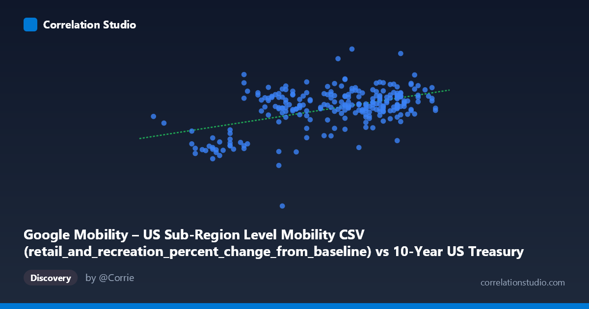
Google Mobility – US Sub-Region Level Mobility CSV (retail_and_recreation_percent_change_from_baseline) vs 10-Year US Treasury Constant Maturity Rate (FRED) (DGS10)
- Pearson correlation (r)
- 0.4892
- Spearman correlation
- 0.3422
- p-value
- 0
- Sample size (n)
- 251
- 95% confidence interval
- 0.3889 to 0.578
- Granger causality
- None
- Granger optimal lag
- 1
AI analysis
Analysis: Treasury Yield vs. Retail & Recreation Mobility (2021)
Relationship Overview
The scatterplot reveals a modest positive relationship between the 10-Year US Treasury Constant Maturity Rate (x-axis) and retail & recreation mobility changes from baseline (y-axis) across US counties during 2021. The linear regression equation (y = 22.90x − 30.46) suggests that higher Treasury yields associate with higher mobility readings, which is intuitively plausible in a recovery narrative: as the economy reopened and strengthened in 2021, both yields and consumer mobility trended upward together. However, the scatter is substantial, with y-values ranging from approximately −38 to +28 percentage points across nearly any given x-value, indicating the relationship is far from deterministic.
Correlation Strength and Statistical Interpretation
The correlation of r = 0.49 is statistically significant (p = 2.22×10⁻¹⁶, N = 16,799), but practical significance requires more careful framing. The R² of 0.239 means that Treasury yield levels explain only about 24% of the variance in retail mobility changes — leaving roughly 76% of variation unexplained by this single predictor. The 95% confidence interval for r [0.389, 0.578] is reassuringly tight, suggesting the true population correlation is reliably moderate but not strong. Critically, the Granger causality tests are non-significant in both directions (X→Y: F = 0.57, p = 0.45; Y→X: F = 0.58, p = 0.45), meaning that neither variable temporally predicts the other at a one-period lag. This firmly discourages any causal interpretation — the co-movement is likely driven by a shared underlying temporal factor rather than a direct predictive mechanism.
Patterns, Clusters, and Outliers
Several structural features stand out in the data. There is a visible central cluster around x ≈ 1.45–1.65 and y ≈ 0–13, consistent with the dominant regime of mid-2021 when yields stabilized and mobility had largely recovered. A distinct lower-left cluster exists near x ≈ 1.05–1.30, where many points show strongly negative mobility values (down to −38.4 at one point), likely corresponding to early 2021 when yields were suppressed and pandemic restrictions remained in effect. That extreme outlier at approximately (1.30, −38.44) warrants specific attention — it likely reflects a county with severe localized restrictions or reporting anomaly. The spread of y-values at any given x-value remains wide throughout, reinforcing the weak-to-moderate nature of the relationship.
Confounding Factors and Caveats
The most important caveat is that both variables are driven primarily by calendar time in 2021 — Treasury yields rose steadily through much of the year as inflation expectations built, while mobility also generally recovered as vaccination rates increased and restrictions lifted. This shared temporal trend creates spurious correlation that the Granger tests correctly flag as non-causal. Additionally, the x-axis data originates from a national-level financial instrument (10-year Treasury yield) being paired against county-level mobility data, creating an ecological mismatch — the yield does not vary by county, so all geographic variation in mobility at a given point in time is attributed to the same yield value. Seasonal effects, regional policy heterogeneity, vaccination rollout pace, and variant waves (particularly Delta in late summer 2021) are all substantial confounders not accounted for here.
Actionable Insights and Further Investigation
Given that the observed correlation is largely a temporal artifact, researchers should consider detrending both series (e.g., using first differences or residuals from a time trend) before re-evaluating the relationship. A multilevel or panel model that accounts for county fixed effects, state-level policy variables, and week-of-year controls would produce a far more reliable estimate of any genuine association. It would also be valuable to test longer lag structures in Granger causality (beyond the optimal lag of 1) and to examine whether the relationship holds within specific mobility categories (e.g., workplace vs. retail) separately. Finally, incorporating vaccination rates, case counts, and consumer sentiment indices as covariates could help isolate whether any residual correlation between financial market signals and behavioral mobility is economically meaningful or purely coincidental.
X dataset: 10-Year US Treasury Constant Maturity Rate (FRED)
Y dataset: Google Mobility – US Sub-Region Level Mobility CSV
Part of experiment: Daily - 10-Year US Treasury Constant Maturity Rate (FRED) vs Google Mobility – US Sub-Region Level Mobility CSV