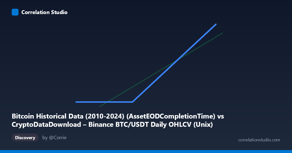
Bitcoin Historical Data (2010-2024) (AssetEODCompletionTime) vs CryptoDataDownload – Binance BTC/USDT Daily OHLCV (Unix)
- Pearson correlation (r)
- 0.9386
- Spearman correlation
- 1
- p-value
- 0
- Sample size (n)
- 3191
- 95% confidence interval
- 0.9343 to 0.9426
- Granger causality
- None
- Granger optimal lag
- 10
- Time coverage
- 2017-08-17 to 2026-05-20
AI analysis
Analysis of Bitcoin Timestamp Correlation
1. What the Visualization Reveals
This scatterplot compares two timestamp columns that both purport to represent completion/recording times for BTC/USDT daily OHLCV data, but from different dataset sources. At face value, since both axes are Unix timestamps tracking the same underlying daily candles, we would expect a near-perfect 1:1 relationship (slope ≈ 1, intercept ≈ 0). Instead, the regression reveals a slope of just 0.00064 — meaning Y barely moves at all as X increases across most of its range. This is a strong signal that something is structurally wrong with one of the two columns rather than evidence of a genuine, meaningful statistical relationship between two independent variables.
2. Strength and Direction of Correlation — With Caveats
The reported r = 0.9386 (r² = 0.881) looks impressive, and the confidence interval [0.934, 0.943] plus p ≈ 0 suggests high statistical confidence. However, this is misleading in context. Look at the sample data: for X values from 2017 through mid-2020 (~1503705600000 to ~1601078400000), Y is essentially frozen at ~1,614,337,xxx — varying only in the last 2-3 digits despite X spanning three years. Then abruptly, starting around X ≈ 1,607,558,400,000 (late 2020), Y begins tracking X almost 1:1 (e.g., X=1733616000000 → Y=1733712385). This is a piecewise/discontinuous pattern, not a linear relationship. The high r² is driven almost entirely by the well-behaved 1:1 segment (2020 onward) dominating the sample size, while the "stuck" early segment contributes mostly noise/flat variance that the linear model partially absorbs. The Granger causality results (p = 0.91 and p = 0.85, no significant direction either way) further confirm there's no meaningful temporal lead-lag dynamic — consistent with these being two representations of the same clock/index rather than causally linked separate phenomena.
3. Notable Patterns and Outliers
The dominant visible feature is a regime break: a large cluster of points where Y is essentially constant (~1.614B) regardless of X value (spanning X from 2017 to ~late 2020), followed by a clean diagonal line where Y ≈ X + ~100,000 seconds from late 2020 onward. This produces a scatterplot that looks like an "L" or hockey-stick shape rather than a classic elliptical correlation cloud. The flat segment is the outlier cluster — likely thousands of rows where Y was populated with a placeholder, default, or erroneously carried-forward timestamp (1,614,337,xxx corresponds to ~Feb 26, 2021) instead of the true completion time.
4. Potential Confounders and Caveats
This is almost certainly a data quality/pipeline artifact, not a substantive relationship. Plausible causes: - A backfill or ingestion job that failed silently for historical dates before ~Nov 2020, defaulting Y to the timestamp of when the backfill script ran (explaining the constant ~1,614,337,xxx value, which decodes to Feb 2021). - Two datasets merged on a join key where only recent rows had valid completion timestamps populated. - The "Y" column may represent metadata (e.g., row-insertion time) rather than true OHLCV close time for older records.
Because of this, the correlation statistic is being computed over a mixture of two populations (broken and working), and r/r² are not meaningfully interpretable as "88% of variance explained" in a scientific sense — the metric is contaminated by the artificial flat segment.
5. Actionable Recommendations
1. Segment the data: Split the analysis at the breakpoint (~Nov 2020) and recompute correlation/regression separately for pre- and post-break subsets. The post-break segment likely shows near-perfect 1:1 correlation (slope ≈1, intercept ≈ small offset), confirming both columns are the same underlying timestamp. 2. Investigate the flat-value cluster: Trace why Y = ~1,614,337,xxx for all early X values — check ETL/ingestion logs around Feb 2021 for a batch job or default-value bug. 3. Do not use this correlation for causal or predictive claims: Given the Granger test shows no lead-lag relationship and the likely data artifact, this pair should not be used to infer any real-world dynamic between "datasets" — it's essentially two copies of a timestamp field with one broken. 4. Data cleaning: Once the bug is identified, re-extract or repair Y for the affected historical rows, then re-run correlation diagnostics to validate true agreement between the two source systems.
X dataset: CryptoDataDownload – Binance BTC/USDT Daily OHLCV
Y dataset: Bitcoin Historical Data (2010-2024)
Part of experiment: Bitcoin - CryptoDataDownload – Binance BTC/USDT Daily OHLCV vs Bitcoin Historical Data (2010-2024)