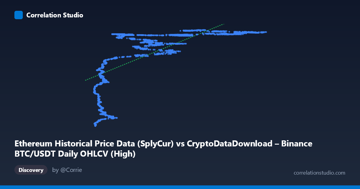
Ethereum Historical Price Data (SplyCur) vs CryptoDataDownload – Binance BTC/USDT Daily OHLCV (High)
- Pearson correlation (r)
- 0.674
- Spearman correlation
- 0.8212
- p-value
- 0
- Sample size (n)
- 3191
- 95% confidence interval
- 0.6546 to 0.6925
- Granger causality
- None
- Granger optimal lag
- 10
AI analysis
Analysis: Ethereum Supply (X) vs. BTC/USDT High Price (Y)
1. What the Visualization Reveals
Despite the labels suggesting an "Ethereum vs. Bitcoin" comparison, the underlying data and behavior strongly suggest this is actually tracking two proxies for the same underlying market trend over time — likely both series are effectively time-indexed (ETH circulating supply grows monotonically with time; BTC price broadly trended upward over the 2017–2026 window). The scatter shows a rapid, non-linear rise in Y at low X values, followed by a plateau — Y jumps from ~94M to ~120M as X moves from ~3,300 to ~20,000, then stays compressed in a tight band (~118M–121M) across the remaining X range up to 126,000. This is a classic logarithmic/saturating curve shape, not a linear one.
2. Strength, Direction, and Statistical Confidence
The Pearson correlation (r = 0.674, r² = 0.454) indicates a moderate positive linear relationship, but only 45% of Y's variance is explained by a straight-line fit to X — the remaining 55% is unexplained by this simple model. The 95% CI [0.655, 0.693] is narrow, and p ≈ 0, meaning the correlation is highly statistically significant and precisely estimated — this is not a fluke of small sample size, but a real, robust pattern given n=3,191. However, statistical significance here reflects the large sample size and strong non-linear trend, not necessarily that a linear model is the right description (see note below). Critically, the Granger causality tests show no predictive direction in either direction (both p-values 0.05, F-stats near/below 1). This tells us that despite the correlation, neither series temporally "leads" the other in a way useful for forecasting — the relationship is likely driven by a shared external trend (time/market cycle) rather than one variable causing movements in the other.
3. Notable Patterns and Non-linearity
The regression note is important: Spearman ρ Pearson r, and the scatter shape (steep rise then plateau) confirms a logarithmic relationship fits better than linear. This pattern — rapid early growth then saturation — is typical of cumulative/supply metrics or price series that have already experienced their major appreciation phase early in the sample window. The tight clustering of Y values (118M–121M) across a huge X range (20,000–126,000) suggests Y is ceiling-bound or in a mature/consolidation phase for most of the dataset, while the sparse, low-X points capture an early, volatile ramp-up phase. This bimodal structure (steep early segment + flat majority) will inflate r² if forced into a linear model and could be a leverage-point artifact — the low-X cluster may disproportionately drive the linear fit.
4. Confounding Factors and Caveats
The most important caveat: X (ETH supply) and Y (BTC price) are both monotonic/trending functions of time, or heavily time-correlated. This is a hallmark of spurious correlation via a common trend — two unrelated time series can show strong r values simply because both drift in the same direction over years. The Granger non-causality result reinforces this: if the relationship were causal, we'd expect at least one direction to show predictive power. Additionally, mixing an Ethereum-supply metric with a BTC price metric conflates two different asset mechanisms — ETH supply is a slow, deterministic/administrative process, while BTC price is driven by speculative demand, making a genuine causal link implausible a priori. Autocorrelation within each series (typical of financial time series and cumulative supply curves) further violates the independence assumptions behind standard p-value calculations, meaning the "p ≈ 0" should be interpreted cautiously.
5. Actionable Insights
1. Re-run correlation using log(X) or a log/power-law transform given the clear saturating shape — this should substantially raise r² beyond 0.454 and better represent the true functional form. 2. Detrend both series first (e.g., first-difference or use % returns instead of levels) before assessing correlation/causality, to remove the shared time trend and test whether any genuine relationship remains. 3. Segment the analysis into the early ramp phase (X < 20,000) vs. the plateau phase — these may represent structurally different regimes (e.g., early network growth vs. mature market) warranting separate models. 4. Given the lack of Granger causality, do not use one series to forecast the other in a trading or predictive model — treat the correlation as descriptive/historical only, not predictive. 5. Investigate whether date/timestamp alignment errors exist, since pairing "ETH supply" with "BTC price" is an unusual combination — confirm the data pipeline correctly mapped intended variables (e.g., was ETH price mistakenly swapped with supply, or is this comparison intentional as a macro/cycle indicator?).
X dataset: CryptoDataDownload – Binance BTC/USDT Daily OHLCV
Y dataset: Ethereum Historical Price Data
Part of experiment: Bitcoin - CryptoDataDownload – Binance BTC/USDT Daily OHLCV vs Ethereum Historical Price Data