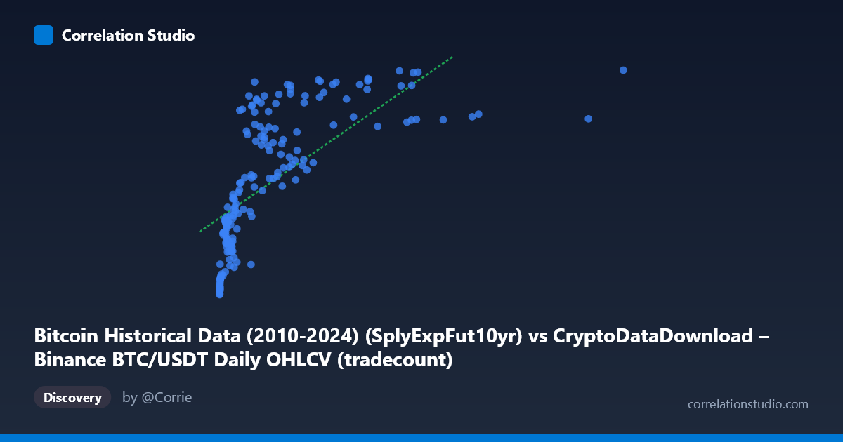
Bitcoin Historical Data (2010-2024) (SplyExpFut10yr) vs CryptoDataDownload – Binance BTC/USDT Daily OHLCV (tradecount)
- Pearson correlation (r)
- 0.6799
- Spearman correlation
- 0.8822
- p-value
- 0
- Sample size (n)
- 180
- 95% confidence interval
- 0.5926 to 0.7514
- Granger causality
- None
- Granger optimal lag
- 10
AI analysis
Analysis: Relationship Between "SplyExpFut10yr" and "Tradecount"
1. What the Visualization Reveals
The scatterplot shows a positive but clearly non-linear relationship between the X variable (labeled SplyExpFut10yr, ranging from ~2,300 to ~10.1 million) and Y (tradecount, ranging from ~20.2M to ~20.8M). The pattern is heavily compressed: the vast majority of points cluster at low X values (under ~3 million), where Y rises steeply and then flattens into an asymptote near 20,750,000–20,800,000 as X grows into the millions. This produces a classic logarithmic or saturating-curve shape rather than a straight line — small increases in X at the low end correspond to large jumps in Y, while the same absolute increase in X at the high end barely moves Y.
2. Strength, Direction, and Statistical Confidence
The Pearson correlation (r = 0.68) indicates a moderately strong positive linear association, with r² = 0.462 meaning the linear model explains only 46% of the variance in Y — leaving more than half unexplained. Given that Spearman's rank correlation exceeds Pearson's r, the true relationship is likely stronger than the linear fit suggests, just not captured well by a straight line; a log or power-law transform of X would likely raise the explained variance substantially. The 95% CI [0.593, 0.751] is reasonably tight and excludes zero, and the p-value (~0) confirms this correlation is not due to chance in this sample. However, the Granger causality tests (p = 0.30 and p = 0.47 for both directions) show no significant temporal predictive relationship — neither variable reliably forecasts future values of the other at the tested lag structure. This is an important caveat: strong contemporaneous correlation does not imply either variable leads or causes changes in the other over time.
3. Notable Patterns and Outliers
- Saturation/plateau effect: Beyond X ≈ 2–3 million, Y values consistently hover in a narrow band (20,650,000–20,800,000), suggesting a ceiling effect or that X's influence diminishes at scale. - Dense low-X cluster: Most data (roughly 70–80% of points) sit below X = 1 million, where the steepest Y growth occurs — this region likely drives most of the linear correlation. - High-leverage outlier: The point at X = 10,085,578 (far exceeding the next-highest values, which cluster near 4–9 million) has substantial leverage on the regression line and warrants a sensitivity check (i.e., refitting without it). - Low-X, low-Y anchor points: Points near X ≈ 2,000–20,000 with Y ≈ 20,209,550–20,260,000 anchor the bottom of the curve, reinforcing the log-like rise.
4. Confounding Factors and Caveats
Both variables are derived from Bitcoin/crypto market data (one appears to be a supply/futures-related metric, the other a trade count), so they may share common underlying drivers — overall market growth, adoption trends, exchange volume expansion, or time itself (since the sample spans 2017–2026, both series may simply trend upward over the study period, creating a spurious or partially spurious correlation via a shared time trend). Without detrending, this correlation may partly reflect autocorrelated growth rather than a genuine causal or structural relationship. Additionally, the "SplyExpFut10yr" label is unusual/ambiguous for OHLCV-derived Bitcoin data — verify that column mapping and units are correct, as mislabeled or transformed fields could distort interpretation. The population (N=3,212) vs. sample (n=180) sampling also means only ~5.6% of available data was used; check that the "every 3rd point" sampling didn't introduce aliasing given any cyclical patterns in the full series.
5. Suggested Next Steps
1. Refit with a log or power transform of X (e.g., ln(X) or X^0.3) to test whether it substantially improves R² — the flattening curve strongly suggests diminishing returns rather than linearity. 2. Detrend both series by time (or run correlation on first differences / returns) to check whether the relationship survives after removing shared temporal drift — this addresses the spurious-correlation risk. 3. Re-run Granger causality with fewer/more lags and using differenced/stationary series, since the current null result may reflect non-stationarity rather than true absence of predictive links. 4. Exclude or separately analyze the extreme outlier (X ≈ 10M) to confirm the curve shape and regression coefficients are stable. 5. Clarify variable definitions (confirm what "SplyExpFut10yr" actually measures) before drawing economic conclusions, since correlation strength and interpretation hinge on correctly understanding what's being compared.
X dataset: CryptoDataDownload – Binance BTC/USDT Daily OHLCV
Y dataset: Bitcoin Historical Data (2010-2024)
Part of experiment: Bitcoin - CryptoDataDownload – Binance BTC/USDT Daily OHLCV vs Bitcoin Historical Data (2010-2024)