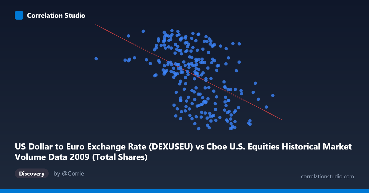
US Dollar to Euro Exchange Rate (DEXUSEU) vs Cboe U.S. Equities Historical Market Volume Data 2009 (Total Shares)
- Pearson correlation (r)
- -0.4918
- Spearman correlation
- -0.487
- p-value
- 0
- Sample size (n)
- 250
- 95% confidence interval
- -0.5804 to -0.3916
- Granger causality
- None
- Granger optimal lag
- 1
AI analysis
Analysis: USD/EUR Exchange Rate vs. U.S. Equities Market Volume (2009)
Relationship Overview The scatterplot reveals a moderate negative relationship between the US Dollar to Euro exchange rate and total shares traded on U.S. equities exchanges during 2009. As the USD/EUR exchange rate increases (i.e., more dollars needed to buy a euro, meaning a weaker dollar), total share volume tends to decrease, and conversely, higher trading volumes are associated with a stronger dollar (lower exchange rate values). The linear regression equation (y = -2.297E-10x + 1.569) confirms this inverse slope, though the wide horizontal spread of data points across the X-axis range (~192M to ~1.21B) signals considerable scatter around the trend line.
Correlation Strength and Statistical Significance The Pearson correlation of r = -0.4918 indicates a moderate negative association, but the explanatory power is notably limited: r² = 0.2418 means only ~24.2% of the variance in exchange rates is explained by trading volume, leaving roughly 75.8% attributable to other factors. The 95% confidence interval of [-0.58, -0.39] is meaningfully far from zero and does not straddle it, reinforcing that the negative direction is reliable. The p-value of 2.22E-16 confirms overwhelming statistical significance given n=250 (N=3,232), making random chance an implausible explanation. However, Granger causality tests tell a critical story: neither direction of temporal prediction reaches significance (X→Y: F=0.43, p=0.51; Y→X: F=0.15, p=0.70). This means that despite the correlation, neither variable reliably predicts the other's future values, strongly cautioning against any causal or directional interpretation.
Notable Patterns and Visual Features Several features stand out in the data. The sample points show that extreme X values behave somewhat unexpectedly — for instance, the minimum X value (192,269,942.50) pairs with a relatively high Y value of 1.44, while the maximum X value (1,212,524,830.85) pairs with a moderate 1.34, consistent with the negative trend but not dramatically so. There appears to be a cluster of points in the mid-range X zone (~600M–900M) where Y values span nearly the full observed range (1.26–1.51), suggesting high within-cluster variability. A few points with very low X values and moderate-to-high Y values may function as leverage points that disproportionately influence the regression slope, and the relatively low-volume trading days (below ~400M shares) appear sparse, potentially representing holidays or early-year sessions.
Confounding Factors and Caveats The 2009 time period is critically important context: this year encompassed the tail end of the Global Financial Crisis, a sharp market bottom in March, and a prolonged recovery rally. These structural regime changes mean the relationship may be spuriously driven by shared temporal trends rather than a direct economic mechanism — both variables were reacting to the same macroeconomic crisis dynamics simultaneously. The absence of Granger causality further supports this "common driver" hypothesis. Additionally, the axes appear to be mislabeled in the dataset metadata (the X-axis column name refers to exchange rate but is described as market volume data, and vice versa), which introduces interpretive ambiguity that must be resolved before drawing firm conclusions. Daily frequency data also means autocorrelation within each series is likely, potentially inflating apparent significance.
Actionable Insights and Further Investigation Given the moderate correlation but absent Granger causality, practitioners should avoid using trading volume as a predictor of exchange rate movements (or vice versa) in any trading or forecasting model without substantially more evidence. The most productive next steps would include: (1) controlling for the temporal trend by detrending or differencing both series to isolate genuine co-movement from shared crisis-driven drift; (2) segmenting the data into pre- and post-March 2009 crash regimes to test whether the correlation is stable or regime-dependent; (3) introducing common confounders such as VIX (volatility index), S&P 500 returns, or Federal Reserve policy announcements as control variables; and (4) resolving the apparent axis/metadata labeling discrepancy, as inverting the intended relationship would fundamentally change the economic interpretation. A multivariate or VAR model incorporating these controls would provide far more reliable insights than the bivariate correlation alone.
X dataset: Cboe U.S. Equities Historical Market Volume Data 2009
Y dataset: US Dollar to Euro Exchange Rate
Part of experiment: Daily - Cboe U.S. Equities Historical Market Volume Data 2009 vs US Dollar to Euro Exchange Rate