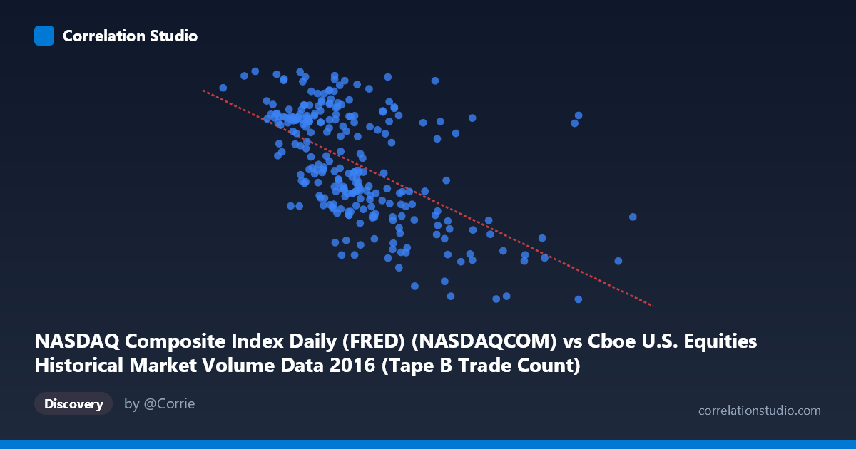
NASDAQ Composite Index Daily (FRED) (NASDAQCOM) vs Cboe U.S. Equities Historical Market Volume Data 2016 (Tape B Trade Count)
- Pearson correlation (r)
- -0.5705
- Spearman correlation
- -0.59
- p-value
- 0
- Sample size (n)
- 252
- 95% confidence interval
- -0.6484 to -0.4809
- Granger causality
- None
- Granger optimal lag
- 10
AI analysis
Analysis: NASDAQ Composite Index vs. Cboe Tape B Trade Count (2016)
Relationship Overview The scatterplot reveals a moderate negative relationship between the NASDAQ Composite Index level and Cboe Tape B trade count throughout 2016. As the NASDAQ index rose to higher levels, the number of trades recorded on Tape B (which covers regional exchange-listed securities) tended to decline. The linear regression equation (y = -0.00178677x + 5558.32) quantifies this inverse slope, suggesting that for every 100,000-point increase in the NASDAQ index, Tape B trade count falls by approximately 179 units. This pattern is visually consistent across much of the data range, though with considerable scatter around the regression line.
Correlation Strength and Statistical Interpretation The Pearson correlation of r = -0.5705 indicates a moderate negative association, and the R² of 0.3255 means that roughly 32.6% of the variance in Tape B trade count is explained by the NASDAQ index level — a meaningful but far from complete explanation, with ~67% of variance attributable to other factors. The 95% confidence interval of [-0.6484, -0.4809] is reasonably tight and does not cross zero, and with a p-value effectively at 0 across a population of N = 3,622, this correlation is statistically robust and unlikely to be a sampling artifact. However, the Granger causality results tell a different story temporally: neither direction (X→Y nor Y→X) shows significant predictive power (F = 0.17, p = 0.998 and F = 0.47, p = 0.911, respectively, at the optimal 10-period lag). This means that while a contemporaneous statistical association exists, neither variable reliably predicts the other's future movements, sharply limiting any causal or forecasting interpretation.
Patterns, Clusters, and Outliers The data exhibits a visible clustering structure. The bulk of observations concentrate in the NASDAQ range of roughly 225,000–400,000, where Tape B trade counts span a wide band from approximately 4,700 to 5,400 — suggesting substantial day-to-day variability even at similar index levels. A distinct group of high-X outliers (NASDAQ values above ~450,000, including one near 558,000 and another near 714,000) consistently show lower trade counts around 4,400–4,600, pulling the regression slope downward and potentially exerting disproportionate leverage on the correlation estimate. On the left tail, lower NASDAQ values (below ~230,000) tend to cluster with higher Tape B counts (5,200–5,487), which is consistent with the inverse trend but also coincides with periods of higher market stress or volatility early in 2016, which are known to drive trading activity.
Confounding Factors and Caveats Several important caveats apply. First, temporal autocorrelation is a major concern: both the NASDAQ index and daily trade counts are time series, and the observed correlation may partly reflect shared secular trends across 2016 (the index trended upward while trading volumes in certain venues shifted structurally) rather than a true functional relationship. Second, Tape B specifically covers securities listed on exchanges other than NYSE and NASDAQ, so its trade count is sensitive to venue fragmentation and routing decisions — factors entirely independent of the NASDAQ index level. Third, macro events (e.g., Brexit in June 2016, the U.S. presidential election in November) likely drove simultaneous spikes in volatility, volume, and index movement, acting as common causes rather than causal links between these two variables. The absence of Granger causality reinforces that the correlation is likely spurious or confounded by shared external drivers rather than mechanistically meaningful.
Actionable Insights and Further Investigation Given the moderate correlation but absent temporal causality, practitioners should avoid using NASDAQ index levels as a predictive signal for Tape B trade routing or volume. Instead, further investigation should explore: (1) decomposing the time series to separate trend, seasonality, and volatility components before re-examining the correlation on residuals; (2) including volatility measures (e.g., VIX) as a covariate, since volatility likely drives both variables simultaneously; (3) examining Tape A and Tape C trade counts to assess whether the inverse relationship is unique to Tape B or a market-wide phenomenon; and (4) testing cross-sectional stability by repeating the analysis on other years to determine whether 2016 is anomalous. The high-leverage outliers at extreme NASDAQ values also warrant closer inspection to confirm they are not data entry errors or exchange-specific anomalies.
X dataset: Cboe U.S. Equities Historical Market Volume Data 2016
Y dataset: NASDAQ Composite Index Daily (FRED)
Part of experiment: Daily - Cboe U.S. Equities Historical Market Volume Data 2016 vs NASDAQ Composite Index Daily (FRED)