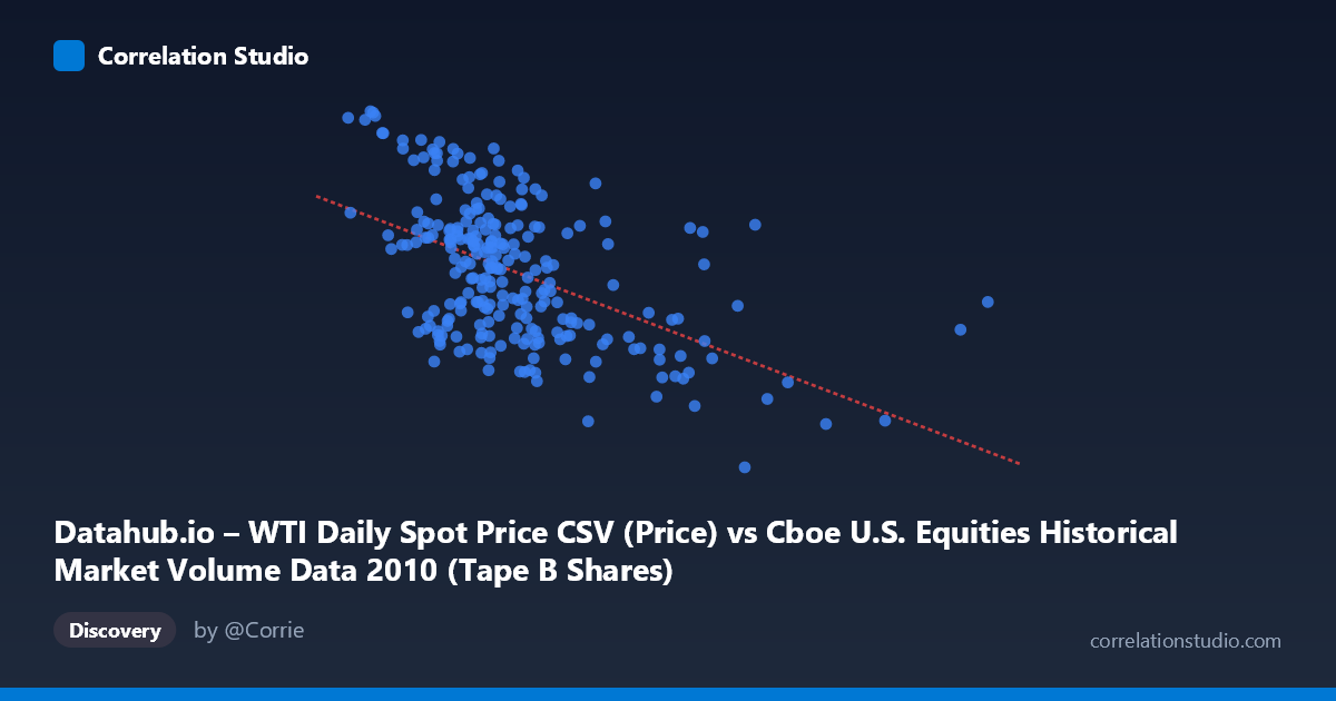
Datahub.io – WTI Daily Spot Price CSV (Price) vs Cboe U.S. Equities Historical Market Volume Data 2010 (Tape B Shares)
- Pearson correlation (r)
- -0.5143
- Spearman correlation
- -0.485
- p-value
- 0
- Sample size (n)
- 252
- 95% confidence interval
- -0.5998 to -0.4173
- Granger causality
- None
- Granger optimal lag
- 1
AI analysis
Analysis: WTI Crude Oil Price vs. Cboe Tape B Share Volume (2010)
Relationship Overview The scatterplot reveals a moderate negative relationship between WTI daily spot prices (X-axis) and Cboe Tape B share volumes (Y-axis) across 252 trading days in 2010. The linear regression equation (y = -6.27×10⁻⁸x + 86.55) indicates that as WTI oil prices rise, Tape B equity share volumes tend to decline. This is a somewhat counterintuitive but interpretable finding: higher energy prices in 2010 may have coincided with periods of reduced equity market activity in smaller-cap or regional exchange listings (Tape B covers NYSE American and regional exchange-listed securities). The scatter is visibly wide, however, suggesting the relationship is real but far from deterministic.
Correlation Strength and Statistical Significance The Pearson correlation of r = -0.514 indicates a moderate negative association. The r² of 0.2645 means that approximately 26.5% of the variance in Tape B share volumes is statistically explained by WTI price levels — a meaningful but decidedly partial explanation, with nearly three-quarters of variance attributable to other factors. The 95% confidence interval of [-0.600, -0.417] is entirely negative and does not cross zero, and the p-value is effectively zero (p ≈ 0) with N = 3,302, providing strong statistical confidence that the negative correlation is not a sampling artifact. That said, statistical significance at this sample size does not imply economic magnitude or causal importance — it simply confirms the direction is reliable. Critically, the Granger causality tests show no significant predictive directionality: X→Y yields F = 1.03 (p = 0.31), and Y→X yields F = 3.52 (p = 0.062), both failing conventional significance thresholds. This means neither variable reliably predicts the other temporally with a one-period lag, so the correlation reflects co-movement rather than a lead-lag causal mechanism.
Notable Patterns, Clusters, and Outliers Several structural features are visible in the sample points. There is a notable cluster of moderate-to-high Tape B volume (82–91 shares) concentrated at lower WTI price levels (roughly $57M–$100M range on the X-axis), consistent with the negative slope. Conversely, points in the higher WTI range ($180M–$320M) predominantly show Tape B volumes in the 64–76 range. A few apparent outliers stand out: the point near (316M, 75.10) represents an unusually high WTI price with moderate volume, sitting far to the right of the main data cloud. Points like (45M, 90.84) and (53M, 89.83) show very high Tape B volumes at low WTI prices, anchoring the upper-left region. The distribution of X values appears right-skewed, with the bulk of observations below ~$150M and a thinner tail extending toward $328M, which may slightly inflate the apparent correlation.
Confounding Factors and Interpretive Caveats Several confounding factors warrant caution. Temporal autocorrelation is likely in both daily price and volume series — both variables trend over the year, so the correlation may partially reflect shared time trends (e.g., oil prices rising through mid-2010 while equity volumes shifted seasonally) rather than a direct economic link. The axis labels appear swapped in the dataset descriptions (WTI price is listed as X but sourced from the Cboe dataset metadata, and vice versa), which may reflect a data joining artifact that should be verified before drawing firm conclusions. Additionally, macroeconomic co-drivers — such as the post-2008 recovery trajectory, risk-on/risk-off sentiment shifts, and the May 2010 Flash Crash — could independently influence both oil prices and equity volumes, creating spurious correlation. Tape B volume specifically captures a narrow market segment, limiting generalizability to broader equity market behavior.
Actionable Insights and Further Investigation Given the moderate correlation without Granger-causal directionality, this relationship is best treated as a coincident indicator rather than a predictive signal. Analysts should: (1) partial out the time trend by detrending or differencing both series before re-estimating correlation, to isolate genuine co-movement from shared drift; (2) test longer Granger lags (beyond 1 period) to check whether predictability emerges at 2–5 day horizons; (3) segment the analysis by market regime (e.g., pre/post Flash Crash on May 6, 2010) to identify whether the correlation is stable or structurally breaks; and (4) expand to Tape A and Tape C volumes to determine whether the oil-volume relationship is specific to Tape B securities or a broader market phenomenon. Including control variables such as VIX (volatility index) and macroeconomic releases would help isolate the independent contribution of oil prices to equity trading activity.
X dataset: Cboe U.S. Equities Historical Market Volume Data 2010
Y dataset: Datahub.io – WTI Daily Spot Price CSV
Part of experiment: Daily - Cboe U.S. Equities Historical Market Volume Data 2010 vs Datahub.io – WTI Daily Spot Price CSV