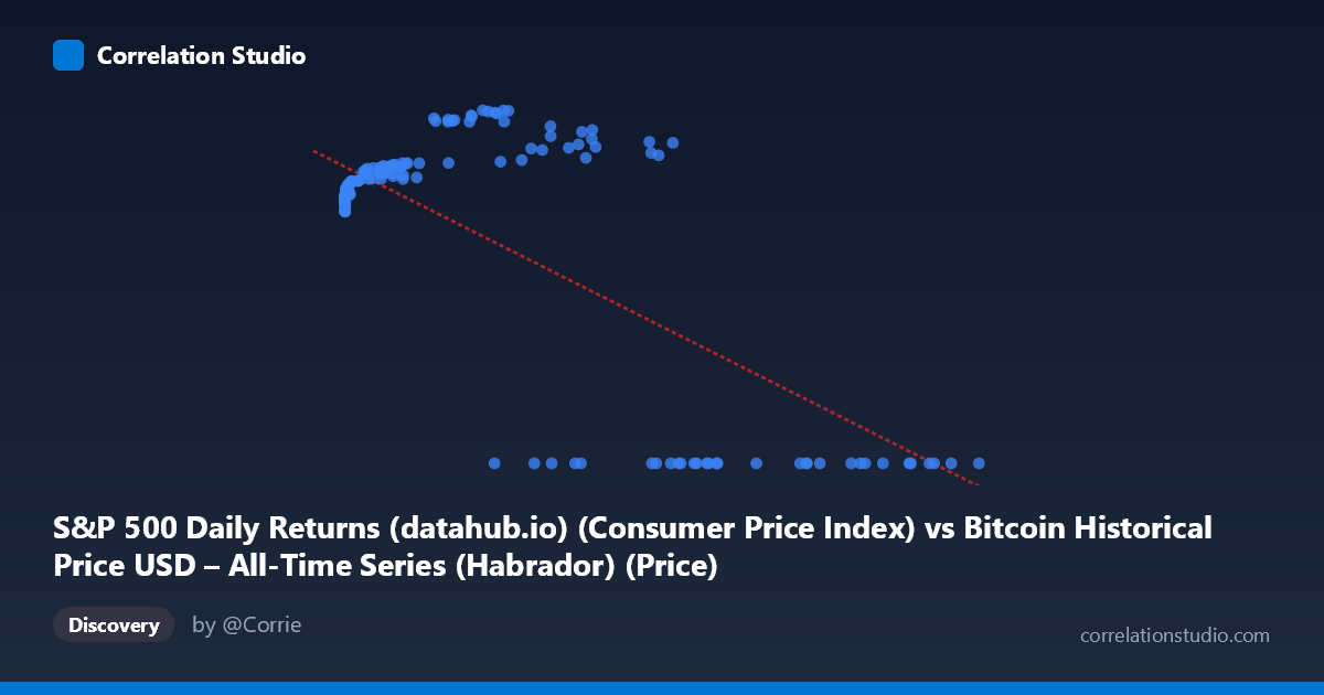
S&P 500 Daily Returns (datahub.io) (Consumer Price Index) vs Bitcoin Historical Price USD – All-Time Series (Habrador) (Price)
- Pearson correlation (r)
- -0.7354
- Spearman correlation
- 0.1008
- p-value
- 0
- Sample size (n)
- 189
- 95% confidence interval
- -0.7947 to -0.6622
- Granger causality
- Y → X
- Granger optimal lag
- 4
AI analysis
Analysis: Bitcoin Price vs. "S&P 500" Column Relationship
Important caveat first: The column labels appear mismatched with their described datasets — the X-axis is labeled as CPI/S&P Daily Returns but contextually behaves like Bitcoin price (range 0.06 to 118,670), while Y-axis (labeled Bitcoin price) behaves like an index bounded 0–306, consistent with a normalized S&P-like series. The interpretation below treats X as the Bitcoin-scale variable and Y as the bounded index, based on the actual numeric behavior in the data.
1. What the Visualization Reveals
The scatterplot shows a non-linear, negative-trending relationship that is actually more complex than the summary statistics suggest. At low X values (under ~1,000), Y clusters tightly between 218–245, rising gently as X increases. Between roughly X = 5,000–60,000, Y climbs further to a peak zone of 260–306. However, at high X values (60,000), Y collapses abruptly to exactly 0.00 in nearly every case. This creates a pattern that looks less like a smooth negative correlation and more like two distinct regimes: a rising phase (low-to-mid X) followed by a hard floor/censoring effect (high X → Y=0).
2. Strength, Direction, and Statistical Confidence
The reported r = -0.7354 (r² = 0.541) indicates a moderately strong negative linear association, with 54% of Y's variance "explained" by X in a linear sense. The tight 95% CI [-0.79, -0.66] and p≈0 confirm this correlation is statistically robust and not a sampling artifact. However, the linear model is misleading here — the negative slope is being driven almost entirely by the cluster of Y=0 points at high X, not by a genuine linear decay across the whole range. The Granger causality results add another layer: Y→X is significant (p=0.023) while X→Y is not (p=0.056), suggesting Y's past values have modest predictive power for future X, but not the reverse — weak evidence of unidirectional temporal precedence, though both p-values are close to conventional thresholds and should be treated cautiously.
3. Notable Patterns and Outliers
- Zero-floor cluster: All X values above ~35,000 (with one exception at 58,724→267.05 and 44,354→287.50) show Y=0.00 exactly — this looks like a data-quality issue (missing/zero-filled values) rather than a true economic relationship. - Rising sub-trend: Excluding the zero cluster, there's actually a positive relationship between X and Y at low-to-mid ranges (X: 0→45,000, Y: 218→306). - Near-zero X outliers: Points like (0.06, 218.44) and (0.20, 218.80) sit at the extreme low end, anchoring the low-Y baseline. - The coexistence of a positive sub-trend and zero-inflated high-X values is what produces the misleading net negative linear fit.
4. Confounding Factors and Caveats
- Zero-inflation bias: The Y=0 cluster at high X values likely reflects missing data, delisting, or an artifact of merging two time series with different active date ranges — not a genuine collapse in value. This alone can flip correlation sign and magnitude. - Metadata mismatch: Column labels/descriptions are swapped or misassigned between datasets, making economic interpretation (Bitcoin vs. CPI vs. S&P 500) unreliable without verification. - Non-stationarity: Both Bitcoin price and equity indices exhibit strong trends/regime shifts over 2010–2026; correlating raw levels (rather than returns) risks spurious correlation from shared trending behavior. - Sample vs. population: n=189 sampled from N=1,865 — confirm sampling was random/representative, especially regarding whether the zero-Y rows are proportionally represented.
5. Suggested Next Steps
1. Verify column/dataset assignment — the labels appear swapped; confirm which series is actually Bitcoin price vs. equity index vs. CPI. 2. Investigate the Y=0 cluster — determine if these are genuine zeros, missing-data placeholders, or a pre-listing period; consider excluding or flagging them separately. 3. Re-run correlation excluding zero-Y rows to see if the true relationship (likely positive) between X and Y emerges. 4. Use returns/log-differences instead of levels to address non-stationarity and reduce spurious correlation risk. 5. Revisit Granger causality after cleaning zero-inflation, since spurious zeros can distort lag-based predictive tests.
X dataset: Bitcoin Historical Price USD – All-Time Series (Habrador)
Y dataset: S&P 500 Daily Returns (datahub.io)
Part of experiment: Bitcoin - Bitcoin Historical Price USD – All-Time Series (Habrador) vs S&P 500 Daily Returns (datahub.io)