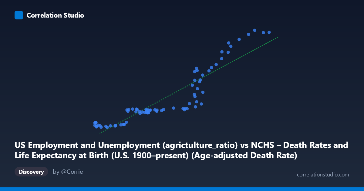
US Employment and Unemployment (agrictulture_ratio) vs NCHS – Death Rates and Life Expectancy at Birth (U.S. 1900–present) (Age-adjusted Death Rate)
- Pearson correlation (r)
- 0.9117
- Spearman correlation
- 0.9379
- p-value
- 0
- Sample size (n)
- 78
- 95% confidence interval
- 0.8646 to 0.943
- Granger causality
- None
- Granger optimal lag
- 10
AI analysis
Analysis: US Agriculture Employment Ratio vs. Age-Adjusted Death Rate
1. Overall Relationship
The scatterplot reveals a strong positive linear relationship between the US agriculture employment ratio (X) and the age-adjusted death rate (Y). As the proportion of employment in agriculture increases, age-adjusted death rates rise correspondingly. The linear regression equation (y = 6.572x − 3,635) suggests that for each unit increase in the agriculture ratio, the death rate increases by approximately 6.57 deaths per 100,000 population. Visually, the data points track closely along the regression line across the full range of both variables, indicating a remarkably consistent association spanning the 1941–2018 observation window.
2. Correlation Strength and Statistical Significance
The correlation is strong (r = 0.911), and the R² of 0.831 indicates that 83.1% of the variance in age-adjusted death rates is explained by the agriculture employment ratio — a substantial proportion for a two-variable model drawn from complex socioeconomic and public health data. The 95% confidence interval for r [0.865, 0.943] is tight and entirely in positive territory, confirming that this association is robustly estimated and not an artifact of sampling variability. The p-value of effectively zero confirms statistical significance at any conventional threshold. However, Granger causality tests find no significant predictive directionality in either direction (X→Y: F = 0.967, p = 0.484; Y→X: F = 0.887, p = 0.552), even at the optimal lag of 10 periods. This is a critical qualification: despite the high correlation, neither variable temporally predicts the other in the Granger sense, strongly suggesting that both are being driven by a common underlying temporal trend rather than a causal mechanism between them.
3. Notable Patterns, Clusters, and Outliers
The data display two somewhat distinct behavioral zones. A lower-left cluster groups densely between agriculture ratios of ~776–1,100 and death rates of ~2,095–3,500, where variance is relatively low and points pack tightly. A sparser upper-right region spans ratios from ~1,300–1,830 and death rates from ~3,400–9,250, where dispersion widens considerably — several points (e.g., (1,743, 9,250), (1,830, 9,100), (1,795, 9,080)) appear as potential leverage points at the high end. A small number of observations near the transition zone (~1,350–1,450 range) show notable vertical spread (death rates ranging from ~3,600 to ~6,500 at similar X values), hinting at a possible non-linear inflection or an era-specific structural break. No extreme outliers distort the overall fit, but the heteroscedasticity — increasing Y-variance at higher X — warrants attention.
4. Confounding Factors and Interpretive Caveats
The most important caveat is that both variables are time-indexed annual series trending in the same historical direction. Agriculture employment ratios declined dramatically over the 20th century as the economy modernized, and age-adjusted death rates declined in parallel due to advances in medicine, sanitation, and public health — entirely independent processes. This is a textbook spurious correlation driven by shared secular trends: two series marching downward together over decades will correlate strongly even when causally unrelated. The absence of Granger causality reinforces this interpretation. Additional confounders include industrialization, urbanization, rising incomes, healthcare access, and nutritional improvements — all of which co-evolved with declining agricultural employment without being captured in this bivariate model.
5. Actionable Insights and Further Investigation
Given the high likelihood of spurious correlation via shared time trends, the most immediate analytical step would be to detrend both series (e.g., first-differencing or HP filtering) and re-examine the correlation on residuals — if r collapses near zero, the association is purely trend-driven. Researchers should also consider multivariate models incorporating confounders such as GDP per capita, urbanization rate, and healthcare expenditure to isolate any residual partial correlation. A structural break analysis around the mid-century period (suggested by the heteroscedasticity in the scatter) could reveal whether the relationship behaves differently across different eras of agricultural and epidemiological transition. Finally, disaggregating by demographic subgroup (race, sex) — given that the death rate data are available by these dimensions — could test whether the association holds uniformly or reflects compositional changes in who comprised the agricultural workforce over time.
X dataset: NCHS – Death Rates and Life Expectancy at Birth (U.S. 1900–present)
Y dataset: US Employment and Unemployment
Part of experiment: Yearly - NCHS – Death Rates and Life Expectancy at Birth (U.S. 1900–present) vs US Employment and Unemployment