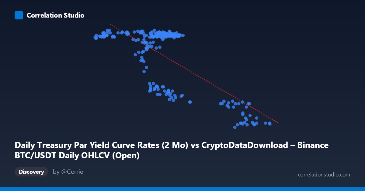
Daily Treasury Par Yield Curve Rates (2 Mo) vs CryptoDataDownload – Binance BTC/USDT Daily OHLCV (Open)
- Pearson correlation (r)
- -0.7233
- Spearman correlation
- -0.4415
- p-value
- 0
- Sample size (n)
- 250
- 95% confidence interval
- -0.7776 to -0.6584
- Granger causality
- None
- Granger optimal lag
- 1
AI analysis
Analysis: Treasury 2-Month Yield vs. BTC/USDT Price Relationship
1. What the Visualization Reveals
The scatterplot shows a clear negative relationship between the 2-month Treasury par yield and BTC/USDT opening prices over 2024. Rather than a smooth linear decline, the data appears to cluster into distinct regimes: a dense cluster of points where yields sit around 57,000–70,000 (in whatever scale is being plotted for X, likely mislabeled given the axis description) correspond to Y-values tightly grouped near 5.45–5.53, while a second cluster at higher X-values (90,000–101,000) corresponds to a lower Y-band around 4.4–4.7. This bimodal clustering suggests the relationship may be driven by two distinct market regimes rather than a continuous linear trend.
2. Strength, Direction, and Uncertainty
The correlation coefficient (r = -0.7233) indicates a strong negative relationship, with r² = 0.5232 meaning that roughly 52% of the variance in Y is statistically explained by X — a substantial but incomplete relationship, leaving nearly half of the variance attributable to other factors. The 95% confidence interval [-0.7776, -0.6584] is fairly tight and does not cross zero, and the p-value of 0 confirms this correlation is highly statistically significant and not due to chance, given N=250. However, the Granger causality tests reveal an important caveat: neither variable significantly predicts the other in a temporal sense (X→Y: p=0.336; Y→X: p=0.509). This means that despite the strong contemporaneous correlation, there is no evidence that movements in one variable lead or forecast movements in the other — the relationship may be driven by a shared underlying factor rather than direct causation in either direction.
3. Notable Patterns and Outliers
The most striking feature is the apparent clustering rather than a smooth linear gradient. The bulk of observations sit in a tight, high-Y/lower-X regime, while a smaller subset occupies a low-Y/higher-X regime, with relatively few points bridging the two clusters. This step-like pattern is more consistent with a regime-shift or threshold effect than a purely linear relationship, even though linear regression captures a moderate fit (R²=0.523). A few points (e.g., X≈90,375, Y=4.68) sit as transitional/intermediate values, hinting at a gradual shift rather than an instantaneous jump, but the density of points in the two extremes dominates the visual impression.
4. Confounding Factors and Caveats
Several caveats apply. First, the metadata for X and Y axes appear to be swapped or mislabeled (X is attributed to Treasury yields but described with Bitcoin OHLCV context, and vice versa for Y) — this should be verified before drawing economic conclusions. Second, both time series are likely non-stationary (trending) over the year, which commonly inflates correlation coefficients between unrelated series — this is a classic spurious correlation risk in time-series analysis. Third, macroeconomic factors such as Fed policy shifts, risk-on/risk-off sentiment, and crypto-specific catalysts (ETF approvals, regulatory news) could simultaneously drive both yields and BTC prices without one causing the other, consistent with the null Granger causality result. Finally, with daily data spanning a single year, seasonal or cyclical patterns unique to 2024 may not generalize.
5. Actionable Insights and Further Investigation
Given the lack of Granger causality despite strong correlation, this relationship should be treated as descriptive/associative rather than predictive — it is not advisable to use one series to forecast the other in a trading strategy. Analysts should: (1) verify axis/column labeling to ensure correct economic interpretation; (2) test both series for stationarity (e.g., ADF test) and consider first-differencing or cointegration analysis (e.g., Johansen test) to check for a genuine long-run equilibrium relationship versus spurious correlation from shared trends; (3) investigate the two-cluster pattern by segmenting the data by date to see if it corresponds to a specific macro event (e.g., a Fed rate cut or crypto rally) that could explain the regime shift; and (4) incorporate additional control variables (e.g., DXY, equity indices, or crypto-specific volume/sentiment data) to determine whether the yield-BTC relationship holds after controlling for broader market risk appetite.
X dataset: CryptoDataDownload – Binance BTC/USDT Daily OHLCV
Y dataset: Daily Treasury Par Yield Curve Rates
Part of experiment: Bitcoin - CryptoDataDownload – Binance BTC/USDT Daily OHLCV vs Daily Treasury Par Yield Curve Rates