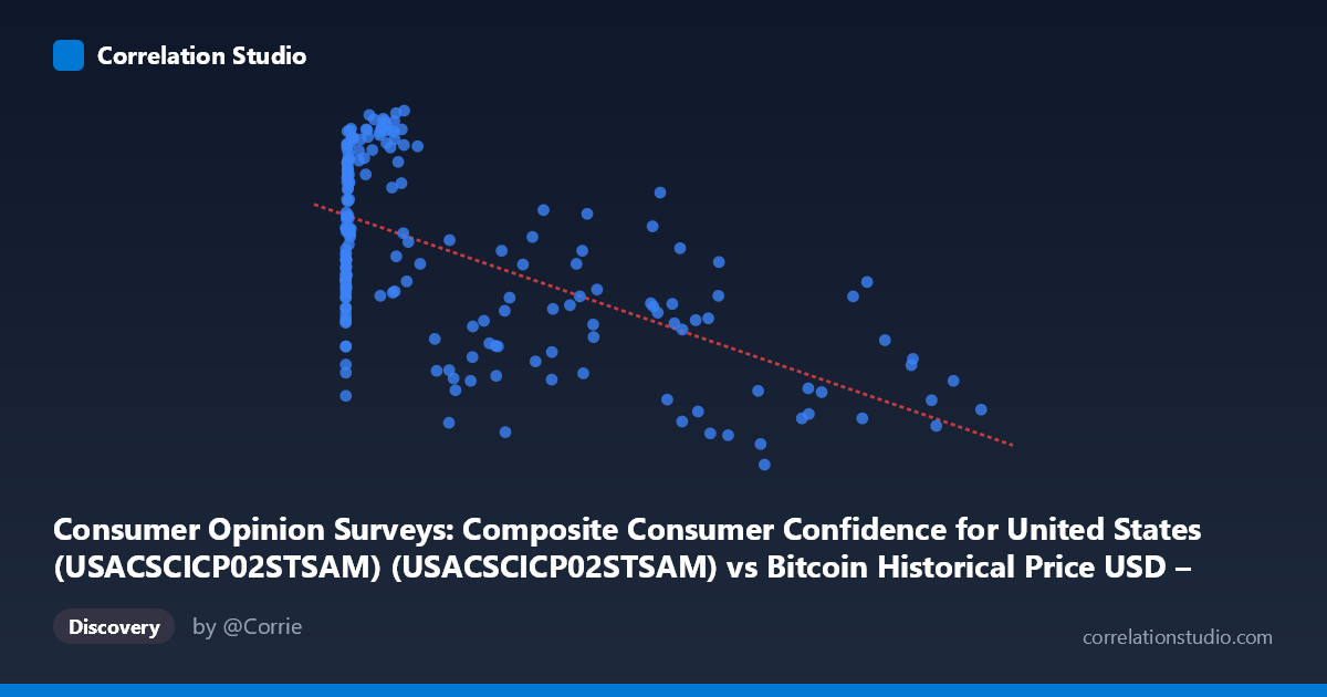
Consumer Opinion Surveys: Composite Consumer Confidence for United States (USACSCICP02STSAM) (USACSCICP02STSAM) vs Bitcoin Historical Price USD – All-Time Series (Habrador) (Price)
- Pearson correlation (r)
- -0.5758
- Spearman correlation
- -0.3231
- p-value
- 0
- Sample size (n)
- 189
- 95% confidence interval
- -0.664 to -0.4719
- Granger causality
- None
- Granger optimal lag
- 1
AI analysis
Analysis: Bitcoin Price vs. Consumer Confidence Index
1. Relationship Overview
The scatterplot displays a moderate negative relationship between Bitcoin's historical USD price (X-axis, heavily right-skewed given the range from $0.06 to $118,670) and the U.S. Composite Consumer Confidence Index (Y-axis, ranging 53.6–109.1). At low Bitcoin prices (sub-$1,000, representing the majority of data points from Bitcoin's early years), consumer confidence values are scattered widely across the full range (65–108), suggesting little direct relationship in this regime. As Bitcoin prices climb into the tens of thousands, confidence readings trend more consistently toward the lower end of the scale (55–80), producing the overall downward slope.
2. Strength, Direction, and Statistical Confidence
The correlation coefficient (r = -0.576) indicates a moderate negative linear relationship, with R² = 0.332 meaning only about 33% of the variance in consumer confidence is explained by Bitcoin price — leaving roughly two-thirds of variation attributable to other factors. The 95% CI [-0.664, -0.472] is reasonably tight and excludes zero, and the p-value (~0) confirms this correlation is statistically robust rather than a chance artifact, despite the modest effective sample size (n=189 paired points from an underlying population of 797). However, the Granger causality tests are critical here: neither variable significantly predicts the other (X→Y: p=0.313; Y→X: p=0.859). This strongly suggests the correlation is not causal in either direction at the tested lag — it's more likely a spurious or confounded relationship driven by shared macroeconomic timing rather than one variable temporally leading the other.
3. Notable Patterns and Outliers
Several structural features stand out: - Heteroscedasticity: variance in Y is much higher at low X values and compresses at high X values, violating simple linear regression assumptions. - Non-linearity: the relationship looks more like a curved/log-decay pattern than a straight line — confidence stays high and volatile while Bitcoin is cheap, then drops and stabilizes lower as price scales into tens of thousands (consistent with bull-market euphoria phases like 2017 and 2021 coinciding with softer confidence readings, and bear-market lows coinciding with higher confidence). - Clustering: a dense cluster of low-price/high-confidence points (early Bitcoin years, 2010–2013) and a separate cluster of high-price/low-confidence points (mature market, 2020s) create a bimodal structure that inflates the linear correlation. - Points like (85,197 → 56.16) and (96,467 → 56.16) and (68,074 → 53.58) anchor the high-price/low-confidence tail, while (313.92 → 105.55) and (997.69 → 105.98) anchor the opposite extreme.
4. Confounding Factors and Caveats
This is a classic case where time is the lurking confound. Both series evolve over a long span (2010–2026) during which Bitcoin underwent multi-order-of-magnitude secular growth while consumer confidence followed its own cyclical macroeconomic path (COVID shock, inflation, rate hikes) unrelated to crypto markets. Regressing two independent time trends against each other routinely produces significant but meaningless correlations. Additionally, the extreme right-skew in X (mean $20,533, stdev $29,894, max $118,670) means the linear regression is dominated by a handful of high-price points, and a log-transform of X would likely be more appropriate and could substantially change the apparent r.
5. Suggested Next Steps
- Re-run correlation on log(X) given the multi-order-of-magnitude spread; this may reveal a cleaner (or weaker) relationship. - Detrend both series (e.g., first-difference or remove long-term trend) before correlating, to test if the relationship holds beyond shared time trends — this is essential given the null Granger results. - Segment by market regime (bull vs. bear cycles) to check if the relationship is regime-dependent rather than continuous. - Treat this correlation as descriptive/associative only — given the lack of Granger causality, it should not be used for predictive or trading purposes linking consumer sentiment to Bitcoin price movements.
X dataset: Bitcoin Historical Price USD – All-Time Series (Habrador)
Y dataset: Consumer Opinion Surveys: Composite Consumer Confidence for United States (USACSCICP02STSAM)
Part of experiment: Bitcoin - Bitcoin Historical Price USD – All-Time Series (Habrador) vs Consumer Opinion Surveys: Composite Consumer Confidence for United States (USACSCICP02STSAM)