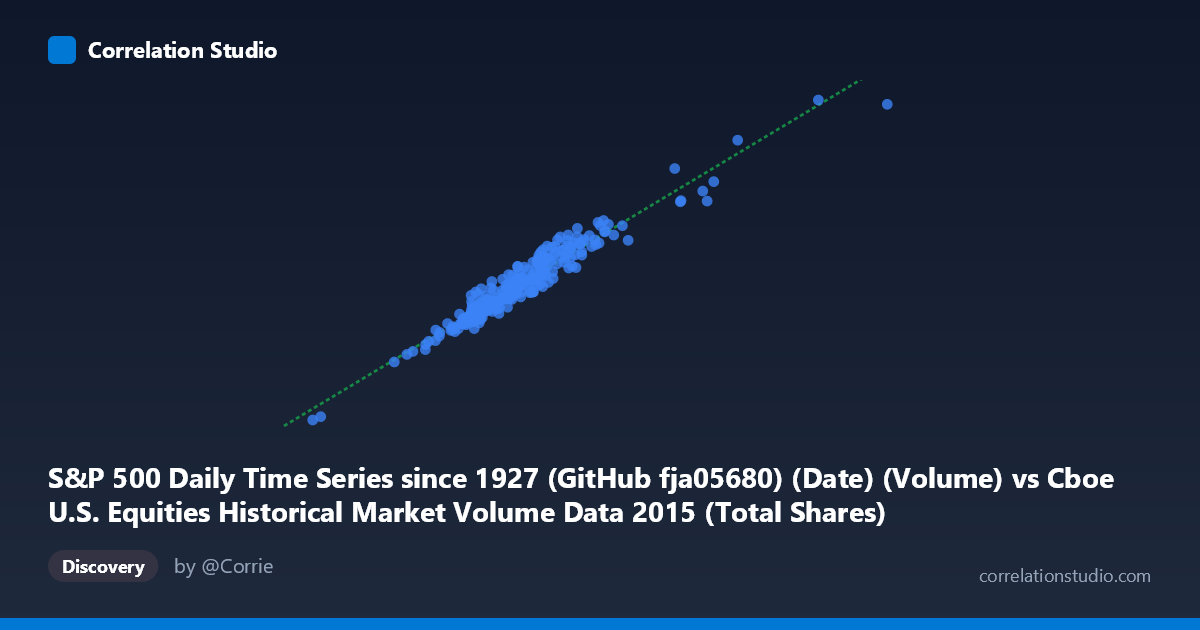
S&P 500 Daily Time Series since 1927 (GitHub fja05680) (Date) (Volume) vs Cboe U.S. Equities Historical Market Volume Data 2015 (Total Shares)
- Pearson correlation (r)
- 0.968
- Spearman correlation
- 0.9574
- p-value
- 0
- Sample size (n)
- 252
- 95% confidence interval
- 0.9591 to 0.9749
- Granger causality
- None
- Granger optimal lag
- 10
AI analysis
Scatterplot Analysis: S&P 500 Volume vs. Cboe U.S. Equities Total Shares (2015)
Relationship Overview
The scatterplot reveals a strong, positive linear relationship between the S&P 500 daily trading volume (X-axis) and the Cboe U.S. Equities total shares traded (Y-axis) across 252 trading days in 2015. As S&P 500 volume increases, total Cboe equity shares rise in a notably consistent, near-linear fashion. The data cloud is relatively tight around the regression line (y = 6.42x + 2.66×10⁸), suggesting that these two volume metrics move in close lockstep throughout the year, which is broadly expected given they both capture daily equity trading activity within the same market ecosystem.
Correlation Strength and Statistical Significance
The correlation is exceptionally strong (r = 0.9680), and the coefficient of determination (r² = 0.9369) indicates that 93.7% of the variance in Cboe total shares is explained by S&P 500 volume — leaving only ~6.3% attributable to other factors. The 95% confidence interval [0.9591, 0.9749] is narrow, reflecting high precision in the estimate, and the p-value of effectively zero confirms this relationship is not a sampling artifact across the n = 252 paired observations drawn from a population of 3,302. However, despite this impressive statistical association, Granger causality tests reveal no significant predictive directionality: neither X→Y (F = 1.63, p = 0.100) nor Y→X (F = 1.85, p = 0.053) clears the conventional significance threshold at a 10-lag structure. This is a critical nuance — knowing today's S&P 500 volume does not reliably predict tomorrow's Cboe total shares beyond what is already captured by the series' own history, and vice versa. The relationship is concurrent rather than temporally predictive.
Notable Patterns, Clusters, and Outliers
The bulk of observations cluster between approximately 420M–570M shares (X) and 2.9B–4.2B shares (Y), forming a dense central core consistent with typical 2015 trading conditions. However, several notable outliers exist at the upper right of the distribution — most prominently a point near (1.09B, 6.68B) and two additional high-volume points around (810M–815M, 5.0B–5.2B) — which likely correspond to episodes of elevated market stress or volatility, such as the August 2015 market correction, when circuit-breaker events and broad sell-offs dramatically amplified volume across all venues simultaneously. At the lower left, a point near (207M, 1.41B) represents an unusually low-volume session. The regression line appears to fit these extremes reasonably well, suggesting the linear model generalizes across market regimes, though leverage from these outliers may be inflating r².
Confounding Factors and Interpretive Caveats
Several important caveats apply. First, both variables are volume-based metrics from the same calendar year and same market, so their co-movement may partly reflect shared exposure to macro drivers — VIX spikes, Fed announcements, earnings seasons, index rebalancing — rather than any structural link between the two series specifically. Second, the Cboe total shares metric aggregates across all U.S. equity exchanges and TRFs, meaning the S&P 500 component is a subset of the denominator, introducing a part-whole relationship that mechanically inflates correlation. Third, the dataset axis labels appear to cross-reference each other's source datasets (S&P 500 data labeling Cboe columns and vice versa), which warrants verification that the variable assignment is correct before drawing firm conclusions. Finally, the 2015 sample includes an extraordinary volatility episode in August, and results may not generalize to other years with calmer or more turbulent conditions.
Actionable Insights and Further Investigation
Given the near-absence of Granger causality, practitioners should not use one series to forecast the other in a trading or risk model — their utility lies in contemporaneous monitoring rather than lead-lag signaling. A worthwhile next step would be to decompose residuals (the unexplained 6.3%) to identify which specific dates deviate from the regression line and whether those deviations correlate with measurable events (VIX level, Fed meeting days, options expiration). Researchers should also test whether this correlation is stable across multiple years or whether the 2015 August shock is disproportionately driving the result. Additionally, given the part-whole concern, replacing the Cboe aggregate with a non-overlapping exchange's volume (e.g., NYSE-only) would provide a cleaner independence test. Finally, a nonlinear or quantile regression analysis could confirm whether the relationship holds uniformly across low-, mid-, and high-volume regimes or whether the upper-tail outliers are driving the linear fit.
X dataset: Cboe U.S. Equities Historical Market Volume Data 2015
Y dataset: S&P 500 Daily Time Series since 1927 (GitHub fja05680) (Date)
Part of experiment: Daily - Cboe U.S. Equities Historical Market Volume Data 2015 vs S&P 500 Daily Time Series since 1927 (GitHub fja05680) (Date)