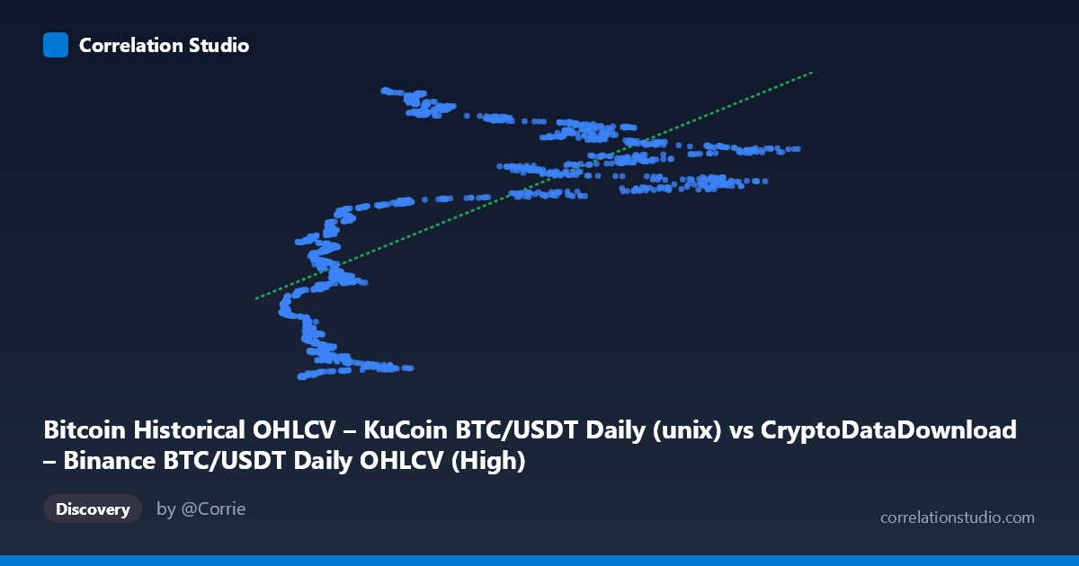
Bitcoin Historical OHLCV – KuCoin BTC/USDT Daily (unix) vs CryptoDataDownload – Binance BTC/USDT Daily OHLCV (High)
- Pearson correlation (r)
- 0.6721
- Spearman correlation
- 0.7498
- p-value
- 0
- Sample size (n)
- 1861
- 95% confidence interval
- 0.6465 to 0.6963
- Granger causality
- None
- Granger optimal lag
- 10
AI analysis
Analysis: Bitcoin Trading Volume vs. Unix Timestamp (Date)
1. What the Visualization Reveals
This scatterplot is somewhat unusual in that the X-axis variable is a timestamp/volume-like metric while Y is essentially a date-encoded price proxy (Unix time of the High price record). Effectively, this plot is showing how a trading metric (X) has trended across Bitcoin's price history from late 2017 through late 2022. The data reveals a moderate positive association: as X increases, Y (representing later dates) also tends to increase, meaning higher values of X are associated with more recent periods in Bitcoin's trading history. The scatter shows clear temporal clustering rather than a clean linear cloud — dense bands of points appear at specific X ranges (e.g., 6,000–10,000 and 40,000–55,000), suggesting these values recur across multiple date clusters corresponding to Bitcoin's cyclical bull/bear market structure.
2. Strength, Direction, and Statistical Confidence
The correlation coefficient (r = 0.672) indicates a moderate-to-strong positive relationship, with r² = 0.452 meaning only 45% of the variance in Y is explained by X — leaving the majority (55%) unexplained by this linear relationship alone. The 95% CI [0.646, 0.696] is tight given the large sample (n=1,861), and the p-value of ~0 confirms the correlation is highly statistically significant and not due to chance. However, statistical significance here reflects sample size more than practical predictive strength — with r² below 0.5, this is a moderate relationship, not a tight one.
Critically, the Granger causality results show no significant predictive direction in either direction (X→Y: p=0.87; Y→X: p=0.088, marginally close to significance but not conclusive at α=0.05). This means neither variable reliably "leads" the other in a time-series forecasting sense, despite the positive correlation. This is an important distinction: correlation captures a static linear association, while Granger causality tests whether past values of one variable improve prediction of future values of the other — here, they largely don't.
3. Notable Patterns and Non-Linear Features
The sample points reveal a non-monotonic, cyclical pattern rather than a simple linear trend. Low X values (3,000–10,000) map to early dates (2017–2020) AND appear again would not — but notably, mid-range X values (40,000–60,000) correspond almost exclusively to the 2021–2022 period (the major bull run), while values in the 20,000–30,000 range map to 2022 dates as well. This suggests Bitcoin's price/volume history is better described as multi-modal or cyclical (accumulation → bull run → correction phases) rather than linear growth. The relationship likely resembles a series of S-curves or plateaus rather than a straight line, which would explain why r² caps around 0.45 despite a "real" underlying relationship — linear regression is a poor functional form for cyclical financial data.
4. Confounding Factors and Caveats
Major caveats apply here: - Autocorrelation: Both variables are time-ordered (daily OHLCV data), meaning consecutive observations are highly non-independent, inflating apparent significance and violating the i.i.d. assumption behind standard p-value calculations. - Cross-exchange proxy issue: X (Binance-based) and Y (KuCoin-based High timestamps) are effectively measuring related but not identical instruments — cross-exchange arbitrage means these series are naturally correlated but the relationship is mechanical/structural rather than causal. - Regime-dependence: The relationship is likely driven entirely by Bitcoin's macro bull/bear cycles (2017 bubble, 2020-21 bull run, 2022 crash) rather than a stable structural relationship — meaning r² and the regression line will not generalize to future, unseen market regimes. - Non-stationarity: Financial time series are typically non-stationary (trending, heteroskedastic), which can produce spurious correlations even after Granger testing.
5. Actionable Insights and Further Investigation
- Detrend/difference the data: Apply first differencing or log-returns transformation to both series before re-testing correlation and Granger causality — this would isolate short-term co-movement from shared long-term trend, which is likely inflating the current r². - Segment by market regime: Split the dataset into bull/bear/accumulation phases and re-run correlation analysis per regime to check if the relationship is stable or regime-specific. - Test non-linear models: Given the apparent cyclical/multi-modal structure, consider polynomial regression, spline fitting, or time-series decomposition (STL) rather than linear regression. - Reconsider variable framing: Since Y is fundamentally a timestamp, this analysis may be better reframed as a straightforward time-series trend analysis of X (e.g., "how has trading volume evolved over Bitcoin's history?") rather than a bivariate correlation study — this would allow use of proper time-series diagnostic tools (ADF tests, seasonal decomposition) instead of Pearson r/Granger causality on what is essentially X vs. time.
X dataset: CryptoDataDownload – Binance BTC/USDT Daily OHLCV
Y dataset: Bitcoin Historical OHLCV – KuCoin BTC/USDT Daily
Part of experiment: Bitcoin - CryptoDataDownload – Binance BTC/USDT Daily OHLCV vs Bitcoin Historical OHLCV – KuCoin BTC/USDT Daily