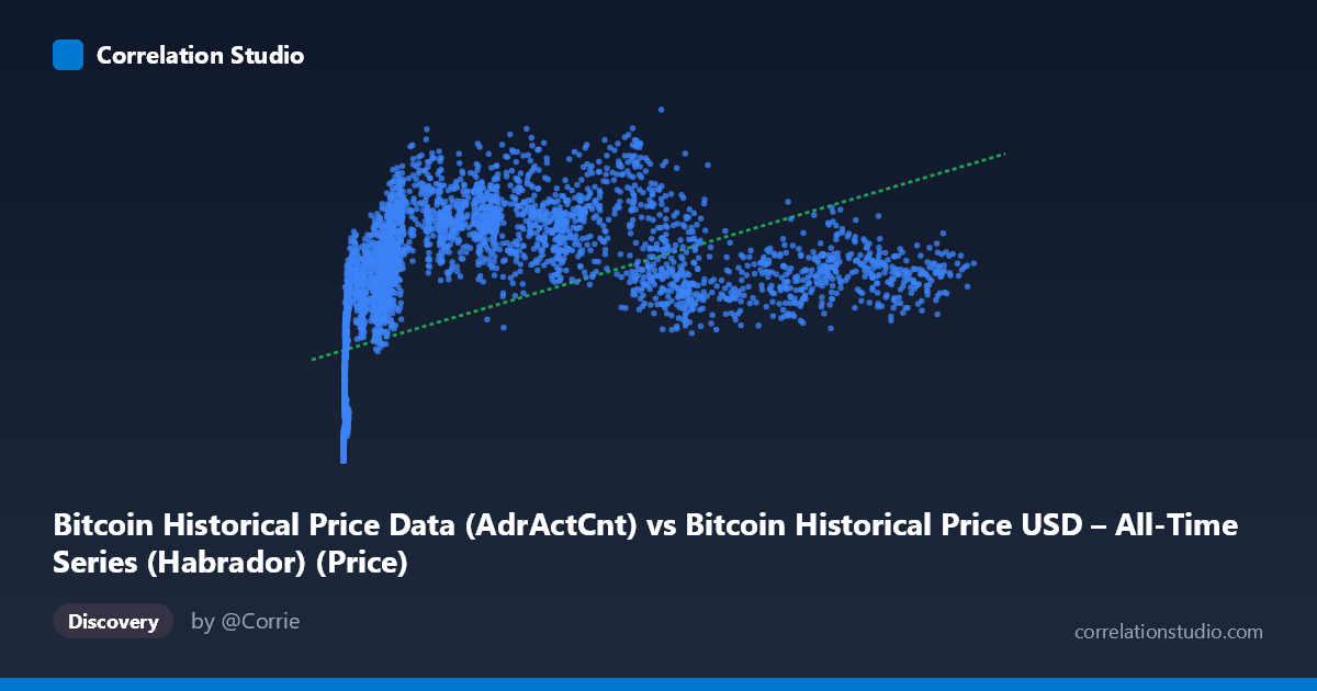
Bitcoin Historical Price Data (AdrActCnt) vs Bitcoin Historical Price USD – All-Time Series (Habrador) (Price)
- Pearson correlation (r)
- 0.4911
- Spearman correlation
- 0.8167
- p-value
- 0
- Sample size (n)
- 5789
- 95% confidence interval
- 0.4713 to 0.5104
- Granger causality
- None
- Granger optimal lag
- 10
- Time coverage
- 2010-07-18 to 2026-05-23
- Recomputed on refreshed data
- 2026-10-24 (r was 0.4927)
AI analysis
Analysis: Bitcoin Active Address Count vs. Price
1. Relationship Overview
The scatterplot depicts Bitcoin's Active Address Count (AdrActCnt) plotted against USD price across nearly the full history of the network (2010–2026). The data shows a clear but non-linear positive relationship: as active addresses increase from near-zero to the tens of thousands, price rises steeply at first, then the relationship flattens and becomes noisy at higher address counts (above ~30,000–50,000). This produces a classic "hockey stick" or logarithmic-style curve rather than a straight line, which is consistent with the note that Spearman's ρ exceeds Pearson's r — the rank-order relationship is stronger than the linear one.
2. Strength, Direction, and Statistical Confidence
The Pearson correlation (r = 0.4927) indicates a moderate positive linear relationship, with r² = 0.2428 meaning only 24.3% of the variance in price is explained by active address count in a linear model — a majority of price variation is driven by other factors. The 95% CI [0.473, 0.512] is tight given the large sample (n=5,764), and the p-value of ~0 confirms this correlation is highly statistically significant and not due to chance. However, statistical significance here should not be conflated with strong predictive power — the modest r² is the more important practical number. Critically, the Granger causality tests show no significant predictive direction in either direction (X→Y: p=0.934; Y→X: p=0.422), meaning that despite the contemporaneous correlation, neither active addresses nor price reliably lead or forecast the other over time at the tested lags. This suggests both variables may be jointly driven by an underlying factor (e.g., overall market cycles, adoption waves) rather than one causing the other in a Granger-testable temporal sense.
3. Notable Patterns and Outliers
Several features stand out: - Saturation/plateau effect: Once active addresses exceed ~30,000–40,000, price shows huge dispersion (from ~$600K to over $1.3M) with little additional explanatory power from address count — this is where the linear model breaks down most visibly. - Low-X cluster: Many early points (X < 20) show very low address counts but already meaningful prices (e.g., ~$1,000–$75,000), reflecting Bitcoin's early years where price appreciation outpaced network usage growth — likely driven by speculation/scarcity rather than utility. - Compression at high X: Points like (94716, 680515) and (120110, 721420) show high address activity but comparatively subdued price relative to (37256, 1257476) — indicating address count alone doesn't distinguish bull-market peaks from consolidation phases. - The overall shape resembles a logarithmic or power-law curve, not a straight line, explaining the linear-vs-rank correlation discrepancy.
4. Confounding Factors and Caveats
This is a time-series correlation of two variables that both trend upward over 16 years, making it highly susceptible to spurious correlation from shared drift/trend (both series are non-stationary). Neither variable is naturally "caused" by the other in the mechanical sense — both are likely responding to a common latent driver: overall market adoption, speculative cycles, macroeconomic liquidity conditions, halving events, and media attention. Address count itself is an imperfect proxy for genuine user adoption (it can be inflated by exchange batching, wallet churn, or on-chain noise unrelated to economic activity). Additionally, using raw (non-detrended, non-differenced) price and address series in a Granger test can produce weak/insignificant results even when the underlying growth trends are related, since Granger causality is best applied to stationary data.
5. Suggested Next Steps
1. Re-fit with a log-log or log-linear model given the clear non-linear/power-law shape — this will likely substantially increase explained variance over the current r²=0.243. 2. Difference or detrend both series (e.g., % change, log returns) before re-running Granger causality tests, since non-stationary trending data can mask or distort true lead-lag relationships. 3. Segment by market regime (bull vs. bear cycles, halving epochs) to see if the X-Y relationship strength/direction changes across phases — the plateau at high address counts suggests regime-dependent behavior. 4. Incorporate additional variables (transaction volume, exchange inflows, macro liquidity/interest rates) to build a multivariate model, since address count alone explains less than a quarter of price variance.
X dataset: Bitcoin Historical Price USD – All-Time Series (Habrador)
Y dataset: Bitcoin Historical Price Data
Part of experiment: Bitcoin - Bitcoin Historical Price USD – All-Time Series (Habrador) vs Bitcoin Historical Price Data