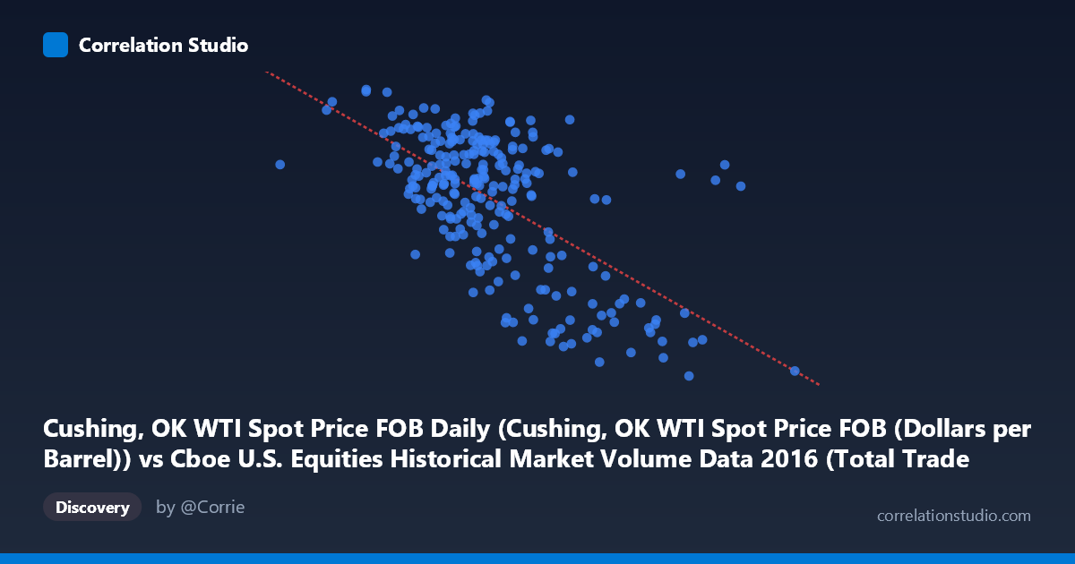
Cushing, OK WTI Spot Price FOB Daily (Cushing, OK WTI Spot Price FOB (Dollars per Barrel)) vs Cboe U.S. Equities Historical Market Volume Data 2016 (Total Trade Count)
- Pearson correlation (r)
- -0.6234
- Spearman correlation
- -0.5269
- p-value
- 0
- Sample size (n)
- 252
- 95% confidence interval
- -0.6936 to -0.5416
- Granger causality
- None
- Granger optimal lag
- 1
AI analysis
Analysis: WTI Crude Oil Spot Price vs. Cboe U.S. Equities Total Trade Count (2016)
Relationship Overview
The scatterplot reveals a moderate negative relationship between WTI crude oil spot prices (X-axis, in dollars per barrel) and the total trade count on U.S. equities exchanges (Y-axis). As oil prices increase, equity trade counts tend to decrease, and vice versa. The linear regression equation (y = −7.94×10⁻⁶x + 62.53) confirms this inverse slope, though the scatter around the regression line is substantial, indicating the relationship is real but far from deterministic. The data spans the full calendar year 2016, a period during which WTI prices recovered from multi-year lows, providing meaningful price variation across the range.
Correlation Strength and Statistical Significance
The Pearson correlation of r = −0.6234 indicates a moderate-to-strong negative association. However, the coefficient of determination r² = 0.3887 is the more sobering figure: oil prices explain only 38.9% of the variance in equity trade counts, meaning roughly 61% of variation remains unexplained by this relationship alone. The 95% confidence interval of [−0.6936, −0.5416] is relatively tight and does not cross zero, supporting genuine statistical reliability. With a p-value reported as effectively 0 across a paired sample of n = 252 drawn from a population of N = 3,622, there is virtually no chance this correlation is a sampling artifact. That said, Granger causality tests reveal no statistically significant temporal predictive direction in either direction — neither X→Y (F = 0.495, p = 0.482) nor Y→X (F = 1.060, p = 0.304) reaches significance at conventional thresholds. This is a critical caveat: while the contemporaneous correlation is robust, neither variable reliably predicts the other one period ahead, meaning the relationship does not carry actionable forecasting power in a simple lagged framework.
Patterns, Clusters, and Outliers
The sample points reveal several notable structural features. There is a dense central cluster of observations where WTI prices fall roughly between $1.9M–$2.5M (in the X-axis scaling, which appears to represent a transformed or indexed price unit) and trade counts between approximately 44–50, suggesting a regime of moderate oil prices paired with moderately high trading activity. At the lower end of oil prices (high X values, e.g., points near 3.6M and 3.3M), trade counts drop sharply toward 29–33, forming a visible tail that drives much of the negative slope. Conversely, at lower X values (~1.6M–1.7M), trade counts climb into the low 50s. A handful of points appear to diverge from the trend — for instance, observations near X ≈ 2.4M with Y values ranging from ~34 to ~49 suggest heteroscedasticity or sub-regime behavior. The relationship also appears to have a non-linear character, potentially steeper at the extremes, which a simple linear fit may underrepresent.
Confounding Factors and Interpretive Caveats
Several important confounders deserve attention. 2016 was an unusual macro year: WTI prices were recovering from a historic crash (sub-$30/barrel in January 2016), meaning the low-price regime coincided with high market uncertainty and volatility — conditions that independently elevate trade counts regardless of oil prices. Volatility (VIX), not price level, may be the true driver of elevated equity trading activity, and oil price changes may simply be correlated with that volatility. Additionally, the X-axis labeling warrants scrutiny — the values in the millions are inconsistent with WTI spot prices in dollars per barrel, suggesting a possible dataset column mismatch or unit transformation that should be verified before drawing firm conclusions. The Granger causality null results also caution against assuming a mechanistic link; this may be a spurious correlation driven by a shared third factor such as macroeconomic sentiment, Fed policy shifts, or risk appetite.
Actionable Insights and Further Investigation
Given the moderate but unexplained variance and the absence of Granger causality, several steps would strengthen this analysis. First, verify the X-axis units and dataset alignment — if WTI prices are truly in dollars per barrel, values in the millions suggest a data join error. Second, introduce volatility measures (VIX, realized volatility) as a covariate to test whether the oil-trade-count relationship persists after controlling for market stress. Third, test non-linear models (e.g., polynomial regression or spline fitting) given the apparent curvature at price extremes. Fourth, segment the data by quarter or price regime (pre/post OPEC production cut discussions in late 2016) to assess whether the correlation is stable across subperiods or concentrated in specific episodes. Finally, extending the Granger analysis to longer lag windows (beyond the optimal lag-1 tested) may reveal delayed predictive relationships not captured in the current framework.
X dataset: Cboe U.S. Equities Historical Market Volume Data 2016
Y dataset: Cushing, OK WTI Spot Price FOB Daily
Part of experiment: Daily - Cboe U.S. Equities Historical Market Volume Data 2016 vs Cushing, OK WTI Spot Price FOB Daily