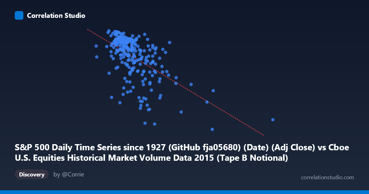
S&P 500 Daily Time Series since 1927 (GitHub fja05680) (Date) (Adj Close) vs Cboe U.S. Equities Historical Market Volume Data 2015 (Tape B Notional)

Pearson correlation (r): -0.5707
Spearman correlation: -0.5618
p-value: 0
Sample size (n): 252
95% confidence interval: -0.6485 to -0.481
Granger causality: None
Granger optimal lag: 7

AI analysis

Analysis: S&P 500 Adjusted Close vs. Cboe Tape B Notional Volume (2015)

Relationship Overview The scatterplot reveals a moderate negative relationship between S&P 500 adjusted closing prices and Cboe Tape B notional trading volume throughout 2015. As the S&P 500 price level increases, Tape B notional volume tends to decrease, and conversely, periods of lower index prices are associated with elevated notional trading activity. This is an intuitively meaningful pattern: market stress and declining prices characteristically trigger heightened trading volumes as investors reposition, hedge, or panic-sell, while calmer, higher-price environments tend to see more subdued activity.

Correlation Strength and Statistical Framing The Pearson correlation of r = -0.5707 indicates a moderate negative association, with the linear regression equation y = -1.80×10⁻⁸x + 2159.32 confirming the downward slope. The R² of 0.3257 means that roughly 32.6% of the variance in Tape B notional volume is explained by the S&P 500 price level — meaningful, but leaving ~67% attributable to other factors. The 95% confidence interval of [-0.6485, -0.4810] is entirely negative and relatively tight, lending confidence that the negative direction is genuine rather than a sampling artifact. The p-value of effectively zero confirms this relationship is highly statistically significant across the 252 paired trading days. However, the Granger causality results are notably absent in both directions — neither X→Y (F=1.92, p=0.067) nor Y→X (F=0.87, p=0.53) clears the significance threshold at the optimal 7-period lag. This means that while the contemporaneous correlation is clear, neither variable reliably predicts the other temporally, cautioning against any mechanistic or causal interpretation.

Notable Patterns, Clusters, and Outliers The sample points reveal important structural features. The bulk of observations cluster in the X range of roughly 3.5–6.5 billion (S&P price × date encoding range), with Tape B notional values tightly bunched between approximately 2,040 and 2,130 — consistent with the S&P 500's relatively narrow trading band for most of 2015. However, there are several pronounced outliers at lower Y values (notional volumes dropping into the 1,867–1,970 range) that correspond to elevated X values, including notably extreme points near X = 12.49–12.58 billion and X = 7.35–7.41 billion. These likely correspond to the August 2015 market correction, when the S&P 500 experienced a sharp sell-off and volatility spiked. A secondary cluster is visible at lower X and higher Y values (~2,125–2,130), representing the quieter, high-price environment of early 2015. The relationship appears somewhat non-linear, with a sharper drop in Y at the extreme high end of X, suggesting threshold or regime-change behavior rather than a clean linear decline.

Confounding Factors and Caveats Several important caveats apply. First, the X-axis appears to encode date information as a numeric timestamp (Unix epoch or similar) rather than a traditional price axis — the axis label references "Date (Adj Close)" which suggests the variable may conflate time with price, making interpretation ambiguous. If X is primarily a proxy for time, the correlation may largely reflect a secular trend (e.g., market declining from mid-year highs through the August correction) rather than a price-volume relationship per se. Second, Tape B specifically covers NYSE American (AMEX) and regional exchange listings, not the full market, so this is a partial volume measure that may not represent aggregate market behavior. Third, macroeconomic events — Federal Reserve interest rate decisions, China volatility spillovers, and oil price movements — all impacted 2015 equity markets simultaneously, acting as common drivers of both price levels and volume. These shared external shocks could be inflating the observed correlation without implying any direct relationship.

Actionable Insights and Further Investigation Practitioners should decompose the X variable to clarify whether it encodes time, price, or both before drawing conclusions — regressing Tape B volume separately against S&P 500 price level and calendar date would disentangle these effects. Given the non-linear appearance of the data, fitting a piecewise or regime-switching model (separating calm vs. stressed market periods) would likely outperform the linear fit and better capture the August correction dynamics. Extending the analysis to full-market consolidated tape volume (not just Tape B) would test whether this relationship generalizes. Finally, incorporating realized volatility (VIX) as a mediating variable is strongly recommended — it likely explains much of the residual 67% variance and may reveal that the price-volume relationship is largely mediated by volatility rather than being direct, which would have meaningful implications for trading strategy and risk management.

X dataset: Cboe U.S. Equities Historical Market Volume Data 2015

Y dataset: S&P 500 Daily Time Series since 1927 (GitHub fja05680) (Date)

Part of experiment: Daily - Cboe U.S. Equities Historical Market Volume Data 2015 vs S&P 500 Daily Time Series since 1927 (GitHub fja05680) (Date)