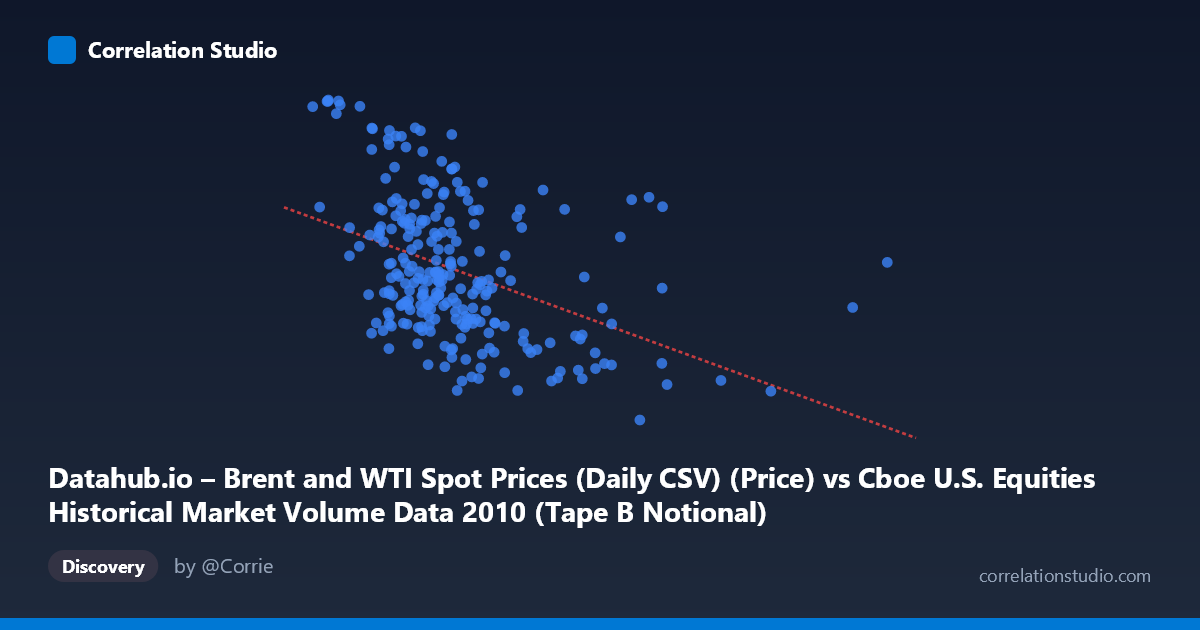
Datahub.io – Brent and WTI Spot Prices (Daily CSV) (Price) vs Cboe U.S. Equities Historical Market Volume Data 2010 (Tape B Notional)
- Pearson correlation (r)
- -0.4224
- Spearman correlation
- -0.4469
- p-value
- 0
- Sample size (n)
- 252
- 95% confidence interval
- -0.5189 to -0.3153
- Granger causality
- None
- Granger optimal lag
- 1
AI analysis
Scatterplot Analysis: Brent Crude Oil Prices vs. Cboe Tape B Notional Volume (2010)
Overall Relationship The scatterplot reveals a moderate negative relationship between Cboe U.S. Equities Tape B notional trading volume (X-axis) and Brent crude oil spot prices (Y-axis) across 252 trading days in 2010. As equity market notional volume increases, oil prices tend to decline — a somewhat counterintuitive pattern at first glance, but one that may reflect broader macroeconomic dynamics during a year marked by post-financial crisis volatility, the European sovereign debt crisis, and the BP Deepwater Horizon oil spill. The linear regression equation (y = -1.208×10⁻⁹x + 85.84) confirms this inverse slope, though the relatively flat gradient suggests the practical magnitude of the effect is modest across the observed volume range.
Correlation Strength and Statistical Significance The Pearson correlation of r = -0.4224 indicates a moderate negative association, but the explanatory power is limited: R² = 0.1785, meaning only 17.8% of the variance in Brent prices is explained by Tape B notional volume. The remaining ~82% is driven by factors entirely outside this model. The result is nonetheless highly statistically significant (p = 2.5×10⁻¹², N = 3,302), making it extremely unlikely this correlation arose by chance. The 95% confidence interval of [-0.52, -0.32] is reasonably tight and excludes zero, confirming the negative direction is reliable. However, statistical significance here is partly a function of the large population size — a correlation this modest would not be considered practically strong in isolation. Critically, the Granger causality tests show no significant predictive directionality in either direction (X→Y: F = 0.83, p = 0.36; Y→X: F = 3.21, p = 0.07), meaning neither variable reliably predicts the other in the subsequent period. This rules out a straightforward temporal lead-lag relationship and cautions against causal interpretation.
Notable Patterns, Clusters, and Outliers Several features stand out in the data. There is a visible cluster of high oil prices (88–93 USD/barrel) concentrated at lower volume levels (roughly below 4×10⁹), suggesting that periods of lower equity trading activity coincided with elevated oil prices — possibly reflecting risk-off sentiment where reduced equity participation accompanied commodity-driven inflation. Conversely, high-volume observations (above 8×10⁹) cluster tightly in the lower price range (67–77 USD/barrel). Three prominent outliers at the upper-right price range — notably the point near (2.0×10⁹, 93.63) and (2.3×10⁹, 93.55) — represent exceptionally high oil prices at very low trading volumes and may correspond to specific geopolitical or seasonal events. The point at approximately (9.8×10⁹, 67.18) anchors the extreme low end of oil prices with high volume. There is also notable vertical spread at mid-range volumes (~4–6×10⁹), suggesting considerable heteroscedasticity and the likely influence of other variables at typical volume levels.
Confounding Factors and Caveats This correlation almost certainly reflects shared dependencies on common macroeconomic drivers rather than any direct causal mechanism between equity notional volume and oil prices. Both variables in 2010 were heavily influenced by: the European sovereign debt crisis (affecting risk appetite and commodities simultaneously), post-crisis Federal Reserve policy (quantitative easing inflating asset prices and commodity demand), the Deepwater Horizon disaster (directly spiking Brent prices mid-year), and seasonal patterns in both energy demand and equity market activity. The dataset swap is also worth noting — the X-axis draws from a Cboe volume dataset while the Y-axis draws from a Datahub oil price dataset, suggesting these may have been paired for exploratory purposes rather than from an established theoretical framework. The optimal lag of only 1 period used in Granger testing may also be insufficient to capture slower-moving macro transmission channels.
Actionable Insights and Further Investigation Despite the lack of Granger causality, the moderate correlation is worth investigating further with multivariate controls. Analysts should consider incorporating VIX (volatility index), S&P 500 returns, USD index, and global demand proxies as control variables to decompose how much of the correlation survives after accounting for shared macro drivers. It would be valuable to segment the year chronologically — pre- and post-Deepwater Horizon, and around key Fed announcements — to test whether the correlation is stable or driven by specific episodes. Extending the analysis to multiple years would test whether this inverse relationship is a 2010-specific artifact or a more persistent structural feature. Finally, given the heteroscedasticity observed at mid-range volumes, a non-linear model or quantile regression may better characterize the tails of this relationship, particularly for risk management applications in portfolio construction involving both equity and energy exposures.
X dataset: Cboe U.S. Equities Historical Market Volume Data 2010
Y dataset: Datahub.io – Brent and WTI Spot Prices (Daily CSV)
Part of experiment: Daily - Cboe U.S. Equities Historical Market Volume Data 2010 vs Datahub.io – Brent and WTI Spot Prices (Daily CSV)