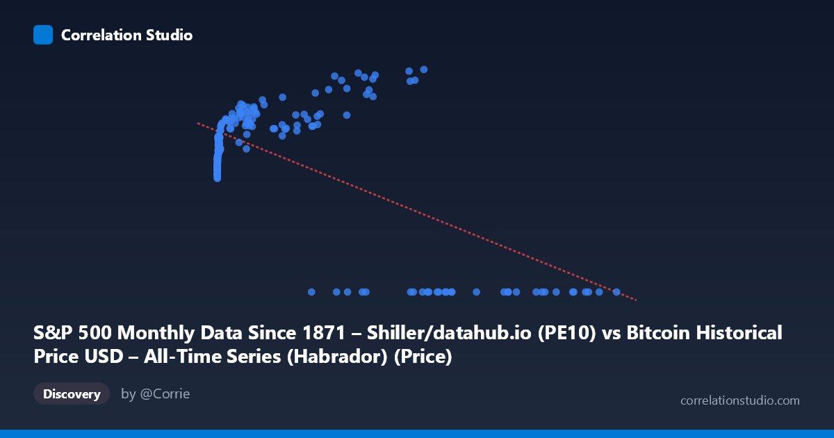
S&P 500 Monthly Data Since 1871 – Shiller/datahub.io (PE10) vs Bitcoin Historical Price USD – All-Time Series (Habrador) (Price)
- Pearson correlation (r)
- -0.638
- Spearman correlation
- 0.0682
- p-value
- 0
- Sample size (n)
- 189
- 95% confidence interval
- -0.7156 to -0.5449
- Granger causality
- Y → X
- Granger optimal lag
- 4
AI analysis
Analysis: Bitcoin Price vs. "PE10" (Mislabeled Series) Relationship
Important caveat first: The column labels appear swapped/mismatched — the X-axis is described as PE10 data but contains values ranging up to 118,670, which corresponds to Bitcoin price data, while Y (bounded 0–38.58) behaves like a bounded ratio/percentage metric. The interpretation below treats the data as presented numerically, but this labeling inconsistency should be resolved before drawing substantive conclusions.
1. What the Visualization Reveals
The scatterplot shows a distinctive non-linear, threshold-like pattern rather than a simple linear trend. At low X values (roughly 0–2,000), Y clusters tightly between 19–30. As X increases into the tens of thousands, Y initially rises further (peaking around 34–38 near X≈35,000–58,000), but then a substantial cluster of points collapses to Y=0 across a wide X range (roughly 27,000–118,670). This creates a bifurcated structure: one regime where Y scales positively with X, and another regime (at high X) where Y drops to zero entirely, regardless of X's magnitude.
2. Strength, Direction, and Uncertainty
The Pearson correlation (r = -0.638, r² = 0.407) indicates a moderate negative linear relationship, but this explains only 40.7% of the variance — meaning nearly 60% of Y's variation is unaccounted for by a linear model with X. The 95% CI [-0.716, -0.545] is reasonably tight and excludes zero, and p≈0 confirms this negative association is statistically robust across the n=189 sample. However, the linear r² masks the true structure: the negative slope is largely an artifact of the "Y=0 cluster" at high X values dragging the regression line downward, not a smooth linear decay. A non-linear or piecewise/threshold model would likely fit dramatically better than the linear r²=0.407 suggests.
The Granger causality results add a temporal dimension: Y Granger-causes X (F=2.617, p=0.037) is significant, while X→Y is marginal (p=0.058). This suggests Y's past values have predictive power for future X values, but not clearly the reverse — implying Y leads X in time, which is an important asymmetry inconsistent with a simple contemporaneous correlation story.
3. Notable Patterns and Outliers
- The zero-Y cluster (X 27,000, Y=0) is the most striking feature — 12+ points sit exactly at Y=0 despite X spanning nearly the entire upper range. This looks like a censoring/missing-data artifact (e.g., Y recorded as 0 when unavailable) rather than a genuine economic zero. - The rising-then-flat arc for X between ~100 and ~60,000 with Y non-zero shows a saturating, logarithmic-like growth curve (Y rises steeply from ~20 to ~38 as X grows from single digits to tens of thousands, then plateaus). - Low-X clustering: the majority of points sit at X<1,000, Y in the 19–30 range, indicating heavy right-skew in X (mean 20,533 vs. median likely far lower), consistent with the huge stdev (29,893) relative to the range.
4. Confounders and Caveats
- Label mismatch: as noted, the axis descriptions don't match the data ranges shown, raising serious doubts about how "X" and "Y" were actually assigned from the two source datasets. This must be clarified before any causal or economic interpretation. - Zero-inflation: the Y=0 cluster likely reflects missing/undefined values (e.g., pre-Bitcoin-existence dates yielding zero price, or PE10 unavailable) rather than true observations — these should be filtered or modeled separately (e.g., via a hurdle/zero-inflated model). - Non-stationarity: both Bitcoin price and equity valuation ratios are highly non-stationary, trending series; Granger causality and correlation on non-stationary time series can produce spurious results unless differenced or detrended. - Time range mismatch: Bitcoin data (2010–2026) is much shorter than Shiller PE10 (since 1871); merging on overlapping dates introduces truncation bias.
5. Suggested Next Steps
1. Verify and correct variable labeling against the raw source files before further analysis. 2. Separate the zero-value cluster and treat as missing data or model with a zero-inflated/two-part regression. 3. Fit a non-linear model (log-log, spline, or piecewise) since the true relationship is clearly not linear — expect r² to improve substantially. 4. Difference or detrend both series and re-run Granger causality to check robustness against non-stationarity artifacts. 5. Investigate the economic mechanism implied by Y leading X — e.g., does equity valuation regime predict subsequent Bitcoin price action, or vice versa — with a clearly specified, correctly-labeled dataset.
X dataset: Bitcoin Historical Price USD – All-Time Series (Habrador)
Y dataset: S&P 500 Monthly Data Since 1871 – Shiller/datahub.io
Part of experiment: Bitcoin - Bitcoin Historical Price USD – All-Time Series (Habrador) vs S&P 500 Monthly Data Since 1871 – Shiller/datahub.io