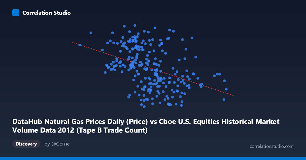
DataHub Natural Gas Prices Daily (Price) vs Cboe U.S. Equities Historical Market Volume Data 2012 (Tape B Trade Count)
- Pearson correlation (r)
- -0.4093
- Spearman correlation
- -0.4551
- p-value
- 0
- Sample size (n)
- 250
- 95% confidence interval
- -0.5076 to -0.3004
- Granger causality
- None
- Granger optimal lag
- 1
AI analysis
Scatterplot Analysis: Natural Gas Prices vs. Cboe Tape B Trade Count (2012)
Relationship Overview The scatterplot reveals a modest negative relationship between Daily Henry Hub Natural Gas Spot Prices (X-axis) and Cboe U.S. Equities Tape B Trade Count (Y-axis) across the 2012 trading year. The linear regression line (y = -4.95×10⁻⁶x + 3.618) slopes downward from left to right, visually confirming the inverse association: as natural gas prices rise, Tape B equity trade counts tend to decline, and vice versa. However, the scatter around this regression line is substantial, suggesting that the linear trend captures only a fraction of what is actually driving trade count variation across this period.
Correlation Strength, Direction, and Statistical Significance The Pearson correlation of r = -0.409 indicates a weak-to-moderate negative relationship. More informatively, r² = 0.167, meaning natural gas prices explain only about 16.7% of the variance in Tape B trade counts — leaving over 83% attributable to other factors entirely. The 95% confidence interval of [-0.508, -0.300] is entirely negative, confirming the direction of the association with reasonable confidence, and the p-value of 1.63×10⁻¹¹ is highly statistically significant given the sample size of n=250 (population N=3,750). However, statistical significance here reflects sample size sensitivity more than practical magnitude. Critically, Granger causality analysis finds no significant temporal predictive direction in either direction (X→Y: F=0.757, p=0.385; Y→X: F=1.952, p=0.164), meaning natural gas prices do not reliably predict future trade counts, nor do trade counts predict future gas prices at a 1-period lag. This absence of Granger causality strongly undermines any causal narrative between these variables.
Notable Patterns, Clusters, and Outliers Several features stand out in the data. The bulk of observations cluster in the X range of roughly 130,000–230,000 (gas price units) with Y values concentrated between 2.2 and 3.2 (trade count), forming a dense central mass. There are visible high-Y outliers — notably points near (152,227, 3.46), (143,080, 3.62), (173,304, 3.61), and (207,237, 3.66) — representing unusually elevated trade counts that sit well above the regression line. Conversely, several low-Y points such as (166,680, 1.82), (226,275, 1.85), and (208,822, 1.87) anchor the lower bound. The far-right outlier at approximately (295,122, 2.44) represents an extreme gas price observation but a middling trade count, exerting potential leverage on the regression fit. The spread of Y values appears somewhat wider at lower X values, hinting at possible heteroscedasticity — variance in trade counts may not be uniform across the gas price range.
Confounding Factors and Interpretive Caveats The most significant caveat is the dataset labeling asymmetry: the X-axis is sourced from the Cboe Market Volume dataset but is labeled as "Natural Gas Prices," while the Y-axis is drawn from the Natural Gas Prices dataset but labeled as "Tape B Trade Count." This cross-dataset column assignment warrants careful verification to ensure the pairing is intentional and meaningful rather than an artifact of column misalignment. Beyond this, both variables are time-series measured daily across 2012, making them susceptible to shared macroeconomic seasonality — equity trading volumes and energy prices can both respond to winter demand cycles, Federal Reserve policy shifts, and broader risk-on/risk-off sentiment without any direct causal link. The absence of Granger causality at lag-1 does not rule out longer-lag relationships or non-linear dynamics. Additionally, Tape B specifically covers NYSE American and regional exchange volumes, which may respond to sector-specific factors (e.g., energy stock trading) that could produce spurious co-movement with gas prices.
Actionable Insights and Further Investigation Given the weak explanatory power and absence of Granger causality, practitioners should not use natural gas prices as a standalone predictor of Tape B trade counts for operational or trading decisions. However, the statistically significant correlation does suggest shared underlying drivers worth exploring. Recommended next steps include: (1) testing longer Granger causality lags (2–10 periods) to detect delayed feedback effects; (2) decomposing both series seasonally to determine whether the correlation persists after removing calendar-driven trends; (3) introducing control variables such as VIX (market volatility), crude oil prices, or broader equity index returns to isolate whether the gas-price/trade-count relationship survives multivariate conditioning; and (4) examining whether the correlation strengthens during specific sub-periods of 2012 (e.g., winter months with energy demand spikes). A non-linear model or quantile regression may also better capture the evident heterogeneity in the scatter, particularly the cluster of high-trade-count outliers that deviate markedly from the linear fit.
X dataset: Cboe U.S. Equities Historical Market Volume Data 2012
Y dataset: DataHub Natural Gas Prices Daily
Part of experiment: Daily - Cboe U.S. Equities Historical Market Volume Data 2012 vs DataHub Natural Gas Prices Daily