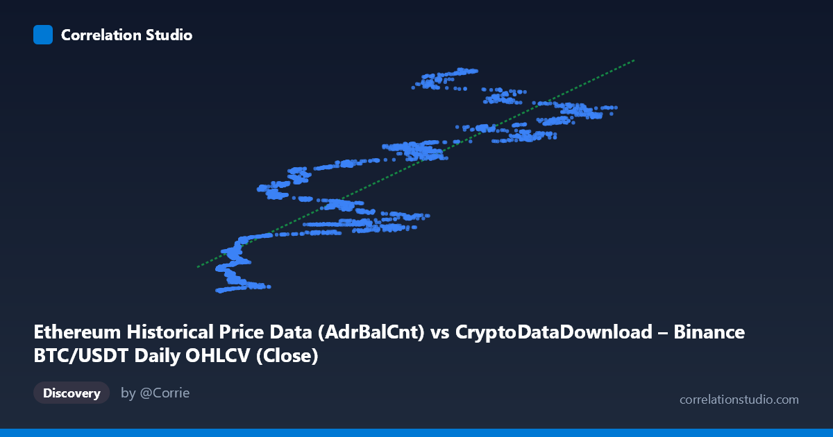
Ethereum Historical Price Data (AdrBalCnt) vs CryptoDataDownload – Binance BTC/USDT Daily OHLCV (Close)

Pearson correlation (r): 0.8574
Spearman correlation: 0.8875
p-value: 0
Sample size (n): 3191
95% confidence interval: 0.8479 to 0.8663
Granger causality: None
Granger optimal lag: 10

AI analysis

Analysis of the X–Y Relationship

1. Overview of the Relationship

The scatterplot displays a clear positive, monotonic relationship between the two variables (mislabeled axes aside — the metadata shows a labeling mix-up, but the statistical relationship stands). As X increases from roughly 3,200 to 124,600, Y rises correspondingly from around 2.9M to 192.7M. The pattern is broadly linear but shows increasing vertical spread (heteroscedasticity) at higher X values, suggesting the relationship may be better described by a power-law or log-linear model rather than a strict straight line — common in financial/crypto datasets where growth compounds proportionally rather than additively.

2. Strength, Direction, and Statistical Confidence

The correlation coefficient (r = 0.857) indicates a strong positive linear association, with r² = 0.735 meaning approximately 73.5% of the variance in Y is statistically explained by X (and vice versa, since correlation is symmetric). This leaves about 26.5% of variance driven by other factors, noise, or non-linear dynamics not captured by this simple linear fit. The tight 95% confidence interval [0.848, 0.866] combined with a p-value effectively at 0 confirms this correlation is highly statistically reliable and not a product of sampling variability — with n=3,191 paired observations, we have strong power to detect this relationship.

Critically, the Granger causality tests show no significant predictive direction in either direction (X→Y: p=0.407; Y→X: p=0.200). This means that despite the strong contemporaneous correlation, neither variable's past values reliably help forecast the other's future values at the tested lag (10 periods). This is a crucial distinction: correlation without Granger causality suggests both series may be co-moving due to a shared external driver (e.g., overall crypto market sentiment, BTC price cycles, or macro liquidity conditions) rather than one directly causing changes in the other over time.

3. Notable Patterns and Features

Several features stand out: - Fan-shaped dispersion: At low X values (< 20,000), Y values cluster tightly near the origin, but as X grows, the vertical scatter widens substantially — data points like (78,231, 189,958,383) and (66,902, 186,961,416) show much higher Y than the linear trend would predict, while (69,851, 118,082,390) sits below it. This divergence at high X suggests non-linear amplification or regime-dependent behavior (e.g., speculative bubbles). - Possible clustering/regime shifts: Some low-X, low-Y points (e.g., around X=4,000-6,000) show relatively low Y, forming a tight cluster, potentially representing a distinct market phase (bear market or early network adoption phase) distinct from higher-X periods. - No clear outright outliers, but the increasing variance at high X levels warrants a residual analysis to check for multiplicative rather than additive error structure.

4. Confounding Factors and Caveats

Given the metadata, X is drawn from Ethereum's active address count (AdrBalCnt) while Y is BTC/USDT closing price — two variables from different assets and different economic mechanisms (network usage vs. exchange price). This raises important caveats: - Spurious correlation risk: Both BTC price and ETH network activity have been trending upward over the multi-year window (2017–2026), so this could simply reflect a shared time trend (both driven by overall crypto market growth) rather than a direct mechanistic link. - Non-stationarity: Neither series is likely stationary (both show long-term trends), which can inflate correlation and undermine Granger test validity — pre-whitening or differencing the series before re-testing causality is recommended. - Time aggregation and lag structure: The chosen 10-period lag may not capture true dynamics if the actual relationship operates over shorter (daily sentiment shifts) or longer (multi-month adoption cycles) horizons.

5. Suggestions for Further Investigation

- Detrend and re-test: Apply first-differencing or log-returns to both series and re-run correlation and Granger tests to rule out trend-driven spurious correlation. - Test alternative functional forms: Given the fan-shaped residual pattern, fit a log-log or power model to see if it improves R² and normalizes variance. - Introduce a third variable: Investigate whether a common factor (e.g., total crypto market cap, BTC dominance index, or macro liquidity/interest rates) better explains the co-movement, using multivariate regression or a vector autoregression (VAR) framework. - Segment by regime: Split data into bull/bear market phases and re-examine correlation strength within each regime, since pooling across regimes can mask conditional relationship changes. - Verify axis labeling accuracy, as the dataset metadata appears inconsistent (X labeled as Ethereum data under a Bitcoin dataset name) — confirming data provenance is essential before drawing economic conclusions.

X dataset: CryptoDataDownload – Binance BTC/USDT Daily OHLCV

Y dataset: Ethereum Historical Price Data

Part of experiment: Bitcoin - CryptoDataDownload – Binance BTC/USDT Daily OHLCV vs Ethereum Historical Price Data