World Bank CO2 Emissions by Country (DataBank) (Total) vs US Employment and Unemployment (unemployed)
- Pearson correlation (r)
- 0.795
- Spearman correlation
- 0.7803
- p-value
- 0
- Sample size (n)
- 80
- 95% confidence interval
- 0.6971 to 0.8638
- Granger causality
- None
- Granger optimal lag
- 10
- Time coverage
- 1941-01-01 to 2020-01-01
AI analysis
Analysis of World Bank CO2 Emissions vs. US Unemployment
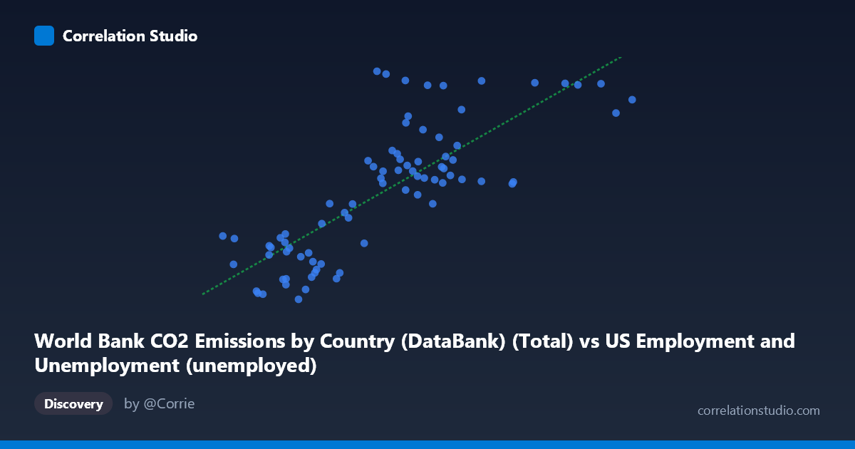
1. Overall Relationship The scatterplot reveals a moderately strong positive association between total CO2 emissions (X-axis, drawn from US Employment data context) and US unemployment figures (Y-axis). The linear regression equation y = 2.39x + 10,684.9 indicates that for every unit increase in CO2 emissions, unemployment rises by approximately 2.39 units. Visually, the data follow a broadly upward trajectory, though with considerable scatter — particularly at mid-to-high X values where the spread widens substantially, suggesting heteroscedasticity and the presence of multiple behavioral regimes within the data.
2. Correlation Strength and Statistical Significance The Pearson correlation of r = 0.795 reflects a moderately strong positive relationship, and the R² = 0.632 means that roughly 63.2% of the variance in unemployment is statistically explained by CO2 emissions within this paired sample. The remaining ~37% is attributable to other factors not captured here. The 95% confidence interval [0.697, 0.864] is notably narrow given n=80, and the p-value ≈ 0 confirms the correlation is highly statistically significant — vanishingly unlikely to arise by chance. However, the Granger causality results are unambiguous in their null finding: neither X→Y (F=0.760, p=0.666) nor Y→X (F=1.073, p=0.401) achieves significance at any conventional threshold, even with an optimal lag of 10 periods. This is a critical qualifier — statistical correlation does not translate into temporal predictive power in either direction, strongly cautioning against any causal interpretation.
3. Notable Patterns, Clusters, and Outliers Several structural features deserve attention: - A dense cluster of points appears in the lower-left quadrant (X: 670–4,000; Y: 9,870–20,000), representing periods of lower emissions and lower unemployment, possibly corresponding to post-WWII or early Cold War decades. - A second diffuse cluster occupies the mid-to-upper range (X: 6,000–10,000; Y: 25,000–42,000), consistent with later industrial expansion periods. - High-leverage outliers are visible at extreme Y values (e.g., points near Y=43,129 at X≈6,001 and Y=41,783 at X≈6,982), which sit well above the regression line and likely correspond to recession years (e.g., early 1980s or 2008–2009 financial crisis). - The upper-right cluster (X: 11,000–14,825; Y: 37,000–41,500) shows high emissions paired with high unemployment, possibly reflecting the 2008–2020 era. - The relationship appears non-linear at higher X values, where the slope flattens, suggesting diminishing marginal association.
4. Confounding Factors and Caveats This correlation almost certainly reflects shared secular trends (both variables trending upward over the 1941–2020 timeframe) rather than any direct mechanistic link between CO2 emissions and unemployment. Key confounds include: - Population growth — a larger population drives both more emissions and a larger labor force with more unemployed persons in absolute terms. - GDP and economic cycles — recessions simultaneously spike unemployment and can temporarily suppress or alter emissions trajectories. - Dataset labeling anomalies — the column metadata is cross-labeled (CO2 data appearing in employment dataset and vice versa), raising data provenance concerns that must be resolved before drawing conclusions. - Spurious correlation via time — both series are annual time-series over 80 years; without differencing or detrending, the r value is likely inflated by the common time trend, which the failed Granger tests partially confirm.
5. Actionable Insights and Further Investigation - Detrend both series (first-differencing or HP filter) before re-running correlation analysis to isolate cyclical co-movement from shared trends — the true relationship may be substantially weaker. - Investigate the outlier years (particularly the extreme high-Y points) to determine whether specific economic shocks (recessions, oil crises) are driving the apparent association. - Disaggregate CO2 by sector (industrial, transport, residential) to test whether any specific emission source correlates more meaningfully with labor market conditions. - Resolve the dataset labeling inconsistency — the axis labels suggest columns may have been joined incorrectly across datasets, which would fundamentally undermine any interpretation. - Consider vector autoregression (VAR) modeling with longer lags or structural break analysis (pre/post-1980) to better characterize the temporal dynamics given the 10-period optimal lag that nonetheless failed Granger significance.
X dataset: US Employment and Unemployment
Y dataset: World Bank CO2 Emissions by Country (DataBank)
Part of experiment: Yearly - US Employment and Unemployment vs World Bank CO2 Emissions by Country (DataBank)