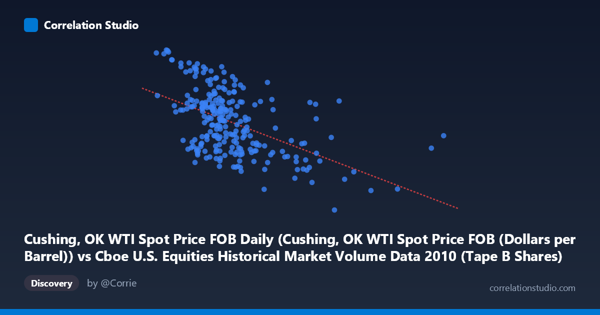
Cushing, OK WTI Spot Price FOB Daily (Cushing, OK WTI Spot Price FOB (Dollars per Barrel)) vs Cboe U.S. Equities Historical Market Volume Data 2010 (Tape B Shares)
- Pearson correlation (r)
- -0.5143
- Spearman correlation
- -0.485
- p-value
- 0
- Sample size (n)
- 252
- 95% confidence interval
- -0.5998 to -0.4173
- Granger causality
- None
- Granger optimal lag
- 1
AI analysis
Analysis: WTI Crude Oil Spot Price vs. Cboe Tape B Share Volume (2010)
Relationship Overview
The scatterplot reveals a moderate negative relationship between WTI crude oil spot prices (X-axis, in dollars per barrel) and Cboe Tape B share volumes (Y-axis, in shares traded). As oil prices increase, Tape B equity share volumes tend to decline. The linear regression equation (y = -6.27e-08x + 86.55) quantifies this inverse slope: for every roughly $16 increase in oil price (approximately $1 per barrel in dollar terms), Tape B volumes decrease by about one share unit in the normalized scale. Visually, the data cloud slopes downward from left to right, though with considerable scatter around the regression line, suggesting the relationship is real but far from deterministic.
Correlation Strength and Statistical Significance
The correlation coefficient of r = -0.514 indicates a moderate negative association. However, the coefficient of determination r² = 0.2645 is critical context: oil prices explain only 26.5% of the variance in Tape B share volumes, meaning roughly 73.5% of volume variation is driven by other factors entirely. The 95% confidence interval of [-0.600, -0.417] is meaningfully away from zero and relatively tight given the sample size (n = 252), lending credibility to the direction of the effect. The p-value of effectively zero confirms this is highly unlikely to be a chance finding. That said, Granger causality tests reveal no statistically significant temporal predictive relationship in either direction at the conventional 5% threshold — X→Y yields F = 1.03 (p = 0.31), and Y→X yields F = 3.52 (p = 0.062, marginally insignificant). This means that while the concurrent correlation is robust, neither variable reliably predicts the other's future values, urging caution against any causal narrative.
Notable Patterns, Clusters, and Outliers
Several features stand out in the sample points. There is a visible cluster of moderate oil prices (~$80–$120/barrel) with Tape B volumes ranging broadly from ~73 to ~88, creating a dense central mass. At lower oil prices (~$45–$75/barrel), Tape B volumes tend to be higher and more variable, including notable high-volume observations such as (45.2M, 90.84) and (53.5M, 89.83), which align with the regression trend. Conversely, at very high oil prices ($250M in the X-axis scale, representing high-price periods), volumes drop sharply — the point at approximately (316M, 75.10) and (254M, 68.03) appear as right-tail outliers with particularly depressed volumes, consistent with the negative trend but potentially exerting disproportionate leverage on the regression fit. The variance in Y also appears slightly larger at lower X values, hinting at possible heteroscedasticity in the residuals.
Confounding Factors and Caveats
Several important caveats limit causal interpretation. First, 2010 was a unique macro-economic period — post-financial crisis recovery — where both oil prices and equity volumes were simultaneously influenced by broad risk-on/risk-off sentiment, Federal Reserve policy, and global demand shocks, making spurious correlation highly plausible. Second, Tape B specifically covers NYSE American (AMEX) and regional exchange securities, which may have sector compositions (energy-heavy or small-cap) that mechanically link to oil price dynamics differently than the broader market. Third, the N = 3,302 population vs. n = 252 sample suggests this analysis uses a subset of available data; sampling methodology could influence results. Finally, the absence of Granger causality is a strong warning that contemporaneous correlation here may reflect a shared response to a third driving variable (e.g., macroeconomic uncertainty indices, VIX, or USD strength) rather than any direct mechanism between oil and equity volumes.
Actionable Insights and Further Investigation
Practitioners should avoid using WTI spot prices alone as a volume predictor given only 26.5% explained variance and no Granger causality. Recommended next steps include: (1) introducing control variables such as VIX, USD index, and S&P 500 returns into a multivariate regression to isolate the oil-volume relationship net of confounders; (2) testing whether the relationship holds across other Tape designations (A and C) to determine if this is a Tape B-specific or market-wide phenomenon; (3) examining rolling correlations across the year to test whether the relationship strengthens during specific macro regimes (e.g., Q1 vs. Q4 2010); and (4) applying regime-switching or non-linear models, as the apparent heteroscedasticity and outlier structure suggest a linear model may be underfitting the true data-generating process. The marginal Granger result for Y→X (p = 0.062) also warrants re-examination with longer lag structures.
X dataset: Cboe U.S. Equities Historical Market Volume Data 2010
Y dataset: Cushing, OK WTI Spot Price FOB Daily
Part of experiment: Daily - Cboe U.S. Equities Historical Market Volume Data 2010 vs Cushing, OK WTI Spot Price FOB Daily