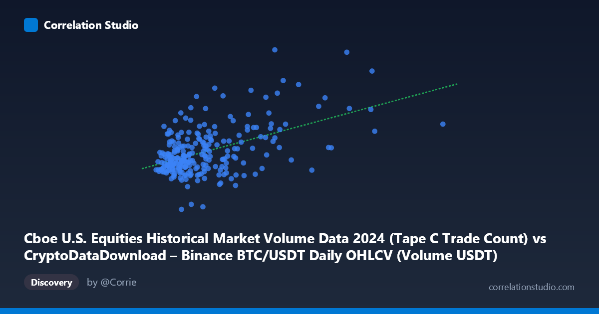
Cboe U.S. Equities Historical Market Volume Data 2024 (Tape C Trade Count) vs CryptoDataDownload – Binance BTC/USDT Daily OHLCV (Volume USDT)
- Pearson correlation (r)
- 0.5058
- Spearman correlation
- 0.3569
- p-value
- 0
- Sample size (n)
- 252
- 95% confidence interval
- 0.4077 to 0.5923
- Granger causality
- None
- Granger optimal lag
- 10
AI analysis
Analysis: Cboe Equities Trade Count vs. Binance BTC/USDT Volume
1. Relationship Overview
The scatterplot displays a modest positive linear relationship between Cboe U.S. equities trade counts (X-axis) and Binance BTC/USDT trading volume in USDT (Y-axis). The data shows a general upward trend—as equity trade counts increase, crypto volume tends to increase as well—but with substantial scatter around the regression line, indicating the relationship is far from deterministic.
2. Strength, Direction, and Statistical Confidence
The correlation coefficient (r = 0.506) indicates a moderate positive relationship, with r² = 0.256 meaning only ~26% of the variance in BTC/USDT volume is explained by equities trade counts—leaving roughly 74% attributable to other factors. The 95% confidence interval [0.408, 0.592] is reasonably tight and excludes zero, and the p-value (effectively 0) confirms this correlation is statistically significant and not due to chance, especially given the n=252 sample size. However, statistical significance should not be conflated with practical predictive strength—a moderate r² means this relationship alone offers limited explanatory power. Critically, the Granger causality tests show no significant predictive direction in either direction (X→Y: p=0.768; Y→X: p=0.863), even at the optimal lag of 10 periods. This is an important caveat: despite the contemporaneous correlation, neither series helps forecast the other over time. This suggests the correlation may reflect a shared external driver (e.g., overall market activity, macroeconomic conditions, or seasonal trading patterns) rather than a lead-lag dynamic between equities and crypto markets.
3. Notable Patterns and Outliers
The bulk of the data clusters in the lower-left region (X: 1-4 billion trades, Y: 1.5-2.2 million volume), reflecting typical daily trading conditions. Several high-leverage outliers are visible at the upper end of the X-axis (e.g., ~6.7B, ~8.6B, ~11B trade counts), which likely correspond to high-volatility or high-activity days (possibly around major market events) and exert disproportionate influence on the regression slope. The relationship also appears heteroscedastic—variance in Y increases somewhat as X grows, and there's no strong evidence of a curved/non-linear pattern; the linear fit seems reasonable but weak. A few low-X, low-Y points (e.g., the point at Y≈1,260,224) suggest occasional quiet days in both markets simultaneously.
4. Confounding Factors and Caveats
Several caveats merit consideration: - Spurious/common-driver correlation: Both series may be independently driven by broader market sentiment, macroeconomic news, or calendar effects (e.g., month-end, quarter-end, or holiday patterns) rather than a direct causal link between equities and crypto trading. - Different market structures: Equity trade counts (Tape C) and crypto volume (USDT-denominated) measure fundamentally different things—one is a count, the other a notional value—making direct economic interpretation tricky. - Non-stationarity: Both time series likely have trends/seasonality that could inflate correlation without true structural relationship; the Granger test controls for this somewhat, reinforcing that the correlation may be non-causal. - Outlier sensitivity: The few very high-X points could be disproportionately driving the r value; robustness checks (e.g., removing top decile) are warranted.
5. Recommendations for Further Investigation
1. Test with detrended/differenced data: Since Granger causality was insignificant on levels, consider re-running on log-returns or first differences to check if a relationship emerges after removing trend/non-stationarity. 2. Identify the outlier dates: Investigate what occurred on the days with extreme X-values (6.7B–11B trades) — these may correspond to known market stress events (e.g., FOMC announcements, ETF approvals) that could explain co-movement. 3. Explore common third factors: Add variables like VIX, overall crypto market cap, or macro news events to test if they better explain the shared variance. 4. Robustness check: Re-run correlation/regression excluding the top 3-5 outliers to assess sensitivity of r and r². 5. Practical takeaway: Given the lack of Granger causality, this correlation should not be used for trading/forecasting purposes in either direction—it's likely coincidental or driven by external factors rather than a tradeable lead-lag relationship.
X dataset: CryptoDataDownload – Binance BTC/USDT Daily OHLCV
Y dataset: Cboe U.S. Equities Historical Market Volume Data 2024
Part of experiment: Bitcoin - CryptoDataDownload – Binance BTC/USDT Daily OHLCV vs Cboe U.S. Equities Historical Market Volume Data 2024