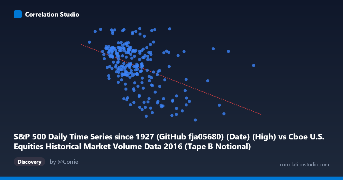
S&P 500 Daily Time Series since 1927 (GitHub fja05680) (Date) (High) vs Cboe U.S. Equities Historical Market Volume Data 2016 (Tape B Notional)
- Pearson correlation (r)
- -0.4475
- Spearman correlation
- -0.4358
- p-value
- 0
- Sample size (n)
- 252
- 95% confidence interval
- -0.5412 to -0.3429
- Granger causality
- None
- Granger optimal lag
- 1
AI analysis
Analysis: S&P 500 Daily High vs. Cboe Tape B Notional Value (2016)
Relationship Overview The scatterplot reveals a negative relationship between the S&P 500 daily high price (X-axis) and Cboe Tape B notional trading volume (Y-axis) across 2016. As the S&P 500 index reached higher price levels, Tape B notional value tended to be lower, and conversely, lower index levels corresponded with higher notional activity. This is a somewhat counterintuitive pattern at first glance — higher market prices correlating with less notional volume on Tape B exchanges — but it reflects the underlying market dynamics of 2016, where early-year volatility and lower price levels drove elevated trading activity, while the later bull-market rally was accompanied by relatively calmer, lower-volume conditions on this particular tape.
Correlation Strength and Statistical Significance The Pearson correlation of r = -0.4475 indicates a moderate negative relationship, with r² = 0.2003, meaning only about 20% of the variance in Tape B notional value is explained by the S&P 500 daily high. While statistically unambiguous — the p-value of 8.19 × 10⁻¹⁴ is far below any conventional significance threshold, and the 95% confidence interval of [-0.54, -0.34] excludes zero comfortably — the practical explanatory power is quite limited. Four-fifths of the variation in Tape B notional activity is driven by factors other than the index price level alone. Critically, the Granger causality tests show no significant predictive direction in either direction (X→Y: F = 0.757, p = 0.385; Y→X: F = 0.113, p = 0.738), meaning neither variable reliably predicts the other at a one-period lag. This rules out a simple lead-lag trading relationship and suggests the correlation is more structural or coincidental than mechanistically causal.
Notable Patterns, Clusters, and Outliers The sample points reveal several important structural features. The bulk of observations cluster in the 3.5–5.5 billion range on the X-axis, where Tape B notional values span a wide range (~2050–2277), suggesting high conditional variability at typical index levels. There are notable outliers at high X values — points near 8.0–8.2 billion (S&P 500 high) that correspond to relatively low notional values (~1890–1920), pulling the regression line downward at the right tail and potentially inflating the apparent negative slope. The point (6,299,758,519; 2272.12) stands out as an anomaly — very high on both axes — and may represent a specific event-driven day. The overall scatter is wide, consistent with the modest r², and there is no strong visual evidence of a clean linear fit; the relationship appears noisy and potentially driven by a handful of extreme observations.
Confounding Factors and Caveats Several important caveats apply. First, the X and Y axis labels appear inverted in the dataset descriptions — the X-axis is labeled as an S&P 500 date column mapped to a "High" value, while the Y-axis refers to Tape B Notional from the S&P dataset, suggesting possible dataset join misalignment or column mapping errors that could distort the interpretation entirely. Second, Tape B notional volume is influenced by share price levels of the specific securities traded on Tape B (NYSE MKT/AMEX-listed stocks), which are structurally different from S&P 500 constituents. Third, 2016 was a structurally unusual year, with the January–February selloff, Brexit shock in June, and the post-election November rally — regime changes that could create spurious correlations when pooled. Finally, the large population (N = 3,622 vs. n = 252 sampled) and daily frequency mean autocorrelation in both time series may inflate statistical significance beyond what independent-sample assumptions would support.
Actionable Insights and Further Investigation Given the limited explained variance and absence of Granger causality, practitioners should not use S&P 500 price levels as a standalone predictor of Tape B notional volume for trading or risk management purposes. More productive next steps would include: (1) segmenting the data by market regime (pre/post-Brexit, pre/post-election) to test whether the negative correlation is regime-specific rather than universal; (2) controlling for the VIX or realized volatility, which likely mediates both variables simultaneously and may account for much of the apparent relationship; (3) verifying dataset alignment to ensure the date joins are correct and no look-ahead or offset bias has been introduced; and (4) exploring non-linear models or quantile regression, since the wide scatter at moderate X values suggests the relationship may be heteroskedastic and poorly captured by OLS. A multivariate approach incorporating volatility, day-of-week effects, and sector rotation would likely yield substantially better explanatory power.
X dataset: Cboe U.S. Equities Historical Market Volume Data 2016
Y dataset: S&P 500 Daily Time Series since 1927 (GitHub fja05680) (Date)
Part of experiment: Daily - Cboe U.S. Equities Historical Market Volume Data 2016 vs S&P 500 Daily Time Series since 1927 (GitHub fja05680) (Date)