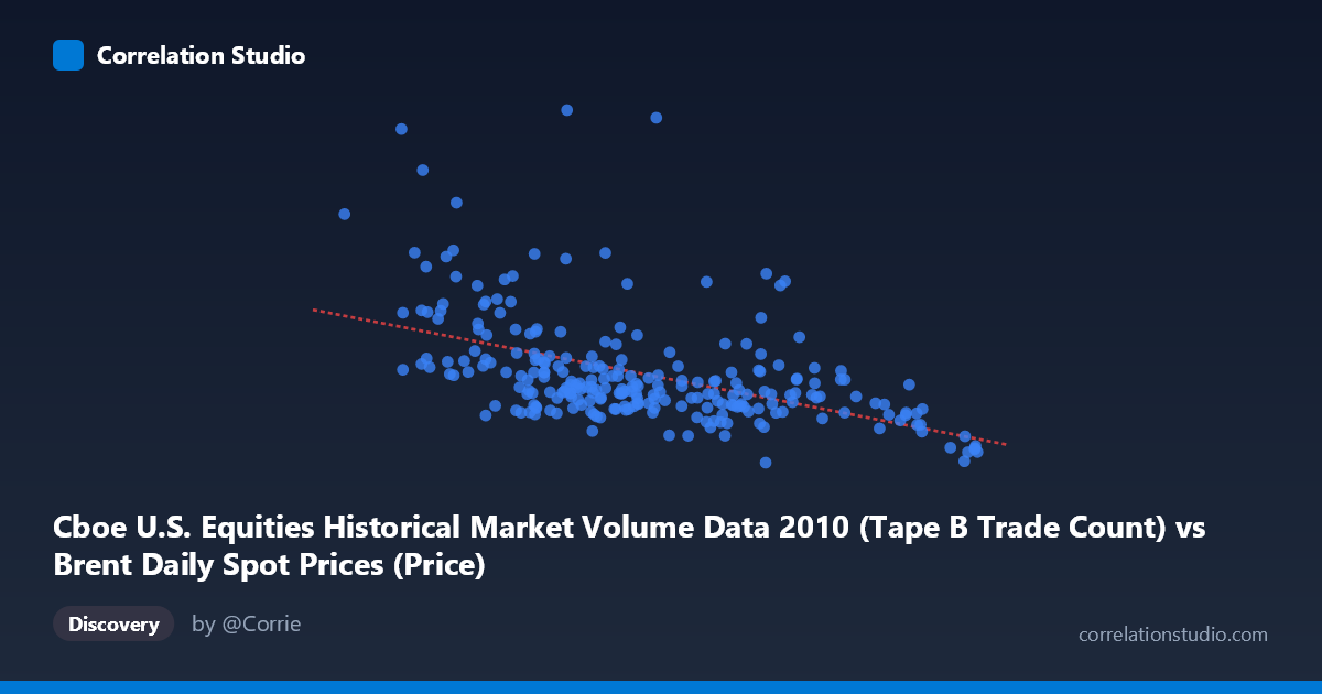
Cboe U.S. Equities Historical Market Volume Data 2010 (Tape B Trade Count) vs Brent Daily Spot Prices (Price)
- Pearson correlation (r)
- -0.4964
- Spearman correlation
- -0.5404
- p-value
- 0
- Sample size (n)
- 252
- 95% confidence interval
- -0.5842 to -0.3972
- Granger causality
- None
- Granger optimal lag
- 10
AI analysis
Scatterplot Analysis: Brent Crude Oil Prices vs. Cboe Tape B Trade Count (2010)
Relationship Overview The scatterplot reveals a moderate negative relationship between Cboe U.S. Equities Tape B trade counts (X-axis, ranging ~67–94 units) and Brent crude oil spot prices (Y-axis, ranging from roughly $96K to $919K in the scaled units shown). The linear regression equation y = -10,853.8x + 1,167,560 captures a downward-sloping trend: as the daily equity trade count increases, Brent crude prices tend to decrease. Visually, this manifests as a loosely dispersed cloud with a discernible negative slope, though substantial scatter around the regression line is immediately apparent, indicating that many data points deviate considerably from this central tendency.
Correlation Strength and Statistical Framing The Pearson correlation of r = -0.4964 indicates a moderate negative association, but the more informative metric is r² = 0.2464, meaning only ~24.6% of the variance in Brent crude prices is explained by Tape B trade counts. The remaining ~75% of variability is driven by other factors entirely. The 95% confidence interval of [-0.5842, -0.3972] is reasonably narrow and sits entirely in negative territory, providing statistical confidence that the true population correlation is genuinely negative. The p-value of effectively zero confirms this is not a chance finding given the large population (N = 3,302). However, the Granger causality results are unambiguous: neither direction (X→Y: F = 0.7524, p = 0.674; Y→X: F = 0.8998, p = 0.534) reaches significance at the optimal 10-period lag, meaning neither variable temporally predicts the other — correlation here carries no detectable causal or predictive temporal structure.
Notable Patterns, Outliers, and Clusters Several features stand out beyond the linear trend. There are clear high-leverage outliers — most notably the point near (76.48, 918,659) and (70.45, 778,566), (67.18, 675,997), and (75.12, 583,091), all of which show low-to-moderate trade counts paired with very high crude prices. These outliers likely exert disproportionate influence on the regression slope and inflate the apparent correlation. There also appears to be a cluster of points concentrated between X = 74–85 and Y = 150,000–400,000, suggesting a dense core of "typical" trading days. The distribution of X is notably right-skewed toward higher trade counts at lower price levels, and there are hints of heteroscedasticity — variance in Y appears larger at lower X values, which violates a key assumption of ordinary least squares regression.
Confounding Factors and Caveats This correlation almost certainly reflects spurious co-movement driven by shared macroeconomic conditions in 2010 rather than any direct mechanism linking equity trade volumes to crude oil pricing. The year 2010 was marked by post-financial-crisis recovery, Eurozone debt concerns, and significant commodity market volatility — all of which simultaneously affected both equity market activity and oil prices through entirely independent channels. The dataset label mismatch is also notable: the X-axis column is labeled as coming from the "Brent Daily Spot Prices" dataset but contains Cboe volume data, and vice versa — this metadata inconsistency warrants verification before drawing any conclusions. Furthermore, Tape B specifically covers regional exchanges (NYSE American, etc.), which may not be the most representative proxy for overall market activity relevant to commodity pricing.
Actionable Insights and Further Investigation Given the absence of Granger causality and the modest r², practitioners should not use Tape B trade counts as a predictive signal for crude oil prices or vice versa. Instead, this analysis suggests several productive next steps: (1) Investigate the outlier dates (particularly the extreme high-Y observations) to determine whether they correspond to specific geopolitical or market events that would explain the anomalies; (2) Test non-linear specifications (logarithmic, polynomial) given the visible heteroscedasticity; (3) Introduce control variables such as VIX (volatility index), USD index, or broader market volume to decompose the confounded relationship; and (4) Expand the Granger causality lag search beyond 10 periods or test with weekly aggregations to rule out longer-horizon predictive relationships. The core takeaway is that while the negative correlation is statistically real, it is economically shallow and temporally non-directional.
X dataset: Brent Daily Spot Prices
Y dataset: Cboe U.S. Equities Historical Market Volume Data 2010
Part of experiment: Daily - Brent Daily Spot Prices vs Cboe U.S. Equities Historical Market Volume Data 2010