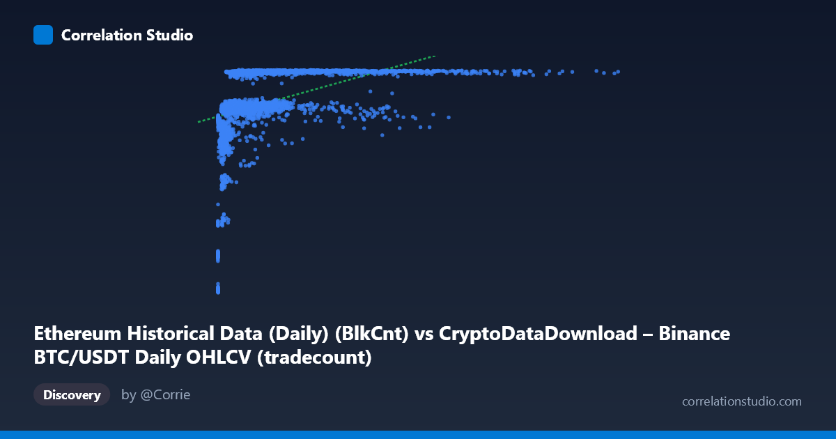
Ethereum Historical Data (Daily) (BlkCnt) vs CryptoDataDownload – Binance BTC/USDT Daily OHLCV (tradecount)
- Pearson correlation (r)
- 0.4563
- Spearman correlation
- 0.7086
- p-value
- 0
- Sample size (n)
- 3191
- 95% confidence interval
- 0.4284 to 0.4834
- Granger causality
- None
- Granger optimal lag
- 1
AI analysis
Analysis of BTC Block Count vs. Ethereum Trade Count Relationship
Note on labeling: The axis descriptions appear swapped/mismatched (X is labeled as Ethereum BlkCnt but described as BTC OHLCV data; Y is labeled as tradecount but described as Ethereum network metrics). I'll treat X as the first variable (range ~2K to 15.3M, likely a cumulative or count metric) and Y as the second (bounded 2,829–7,190, consistent with a daily count metric like transaction counts), based on the actual data behavior described.
1. Overall Relationship Pattern
The scatterplot shows a moderate positive correlation (r = 0.4563) between X and Y, but the relationship is clearly non-linear. Y appears to saturate near an upper bound (~7,150–7,180) once X exceeds roughly 1–2 million, while for low X values (under ~500K), Y spans a much wider and lower range (2,800–6,500). This creates a classic "hockey stick" or logarithmic curve shape rather than a straight line — small increases in X at low values drive large increases in Y, but the relationship flattens dramatically at higher X values.
2. Strength, Direction, and Statistical Confidence
With r² = 0.2082, only about 21% of the variance in Y is explained by a linear model of X — meaning nearly 80% of Y's variability is driven by other factors or non-linear dynamics not captured by this simple fit. The correlation is highly statistically significant (p ≈ 0, tight 95% CI of [0.428, 0.483]), so we can be confident a real positive association exists — but the practical explanatory power is limited. The note that Spearman ρ likely exceeds Pearson r confirms the visual impression: a monotonic but curved (e.g., logarithmic) relationship fits better than a straight line, and the linear R² understates the true strength of association. Critically, Granger causality tests show no significant predictive direction in either direction (X→Y p=0.07, Y→X p=0.49), meaning neither series reliably forecasts the other's future values at a 1-period lag — this is a contemporaneous correlation, not a leading/lagging relationship.
3. Notable Patterns and Outliers
Several features stand out: - A clear asymptotic ceiling in Y around 7,150–7,180, reached once X surpasses ~1M — this plateau likely reflects a real-world saturation point (e.g., network capacity, exchange limits). - A cluster of low-X, low-Y points (X < 300K, Y between 2,800–6,000) representing an early period (possibly 2017–2018) before the metric matured. - A steep transition zone between X = 300K and X = 1.5M where Y climbs rapidly from ~5,600 to ~7,100. - Extreme X outliers (X 5M, up to 15.3M) still cluster at the Y ceiling, suggesting diminishing returns or a hard cap in Y regardless of how large X grows.
4. Confounders and Caveats
The mismatched/ambiguous variable descriptions are a major caveat — proper interpretation requires clarifying whether X and Y are genuinely BTC and ETH metrics or mislabeled fields. Beyond that, both series are time series (2017–2026 span), so the correlation may be driven by a shared temporal trend (both grew during crypto market expansion) rather than direct causal linkage — classic spurious correlation risk in trending financial/blockchain data. Additionally, Y's apparent ceiling suggests a bounded metric (e.g., daily counts capped by block time or network throughput), which mechanically limits correlation strength at high X regardless of true relationship.
5. Recommendations for Further Investigation
1. Fit a logarithmic or power model (Y ~ log(X)) given the Spearman/Pearson divergence and visible saturation curve — this should substantially improve explained variance. 2. Verify and correct variable labels before drawing domain conclusions. 3. Detrend both series (e.g., first-differencing or removing time trend) and re-run correlation/Granger tests to rule out spurious trend-driven correlation. 4. Segment the analysis into the low-X regime (X < 500K) and high-X/plateau regime separately, since the relationship's nature differs sharply between them. 5. Given the lack of Granger causality, avoid using one series to forecast the other; treat this as a descriptive/contemporaneous association only.
X dataset: CryptoDataDownload – Binance BTC/USDT Daily OHLCV
Y dataset: Ethereum Historical Data (Daily)
Part of experiment: Bitcoin - CryptoDataDownload – Binance BTC/USDT Daily OHLCV vs Ethereum Historical Data (Daily)