17-Year Expected Inflation (EXPINF17YR) | FRED | St. Louis Fed (EXPINF17YR) vs FRED – Copper Price (Global) (PCOPPUSDM)
- Pearson correlation (r)
- -0.5978
- Spearman correlation
- -0.5762
- p-value
- 0
- Sample size (n)
- 417
- 95% confidence interval
- -0.6562 to -0.5324
- Granger causality
- None
- Granger optimal lag
- 1
- Time coverage
- 1992-01-01 to 2026-09-01
- Recomputed on refreshed data
- 2026-10-27 (r was -0.6151)
AI analysis
Analysis: Copper Price vs. 17-Year Expected Inflation
1. Relationship Overview
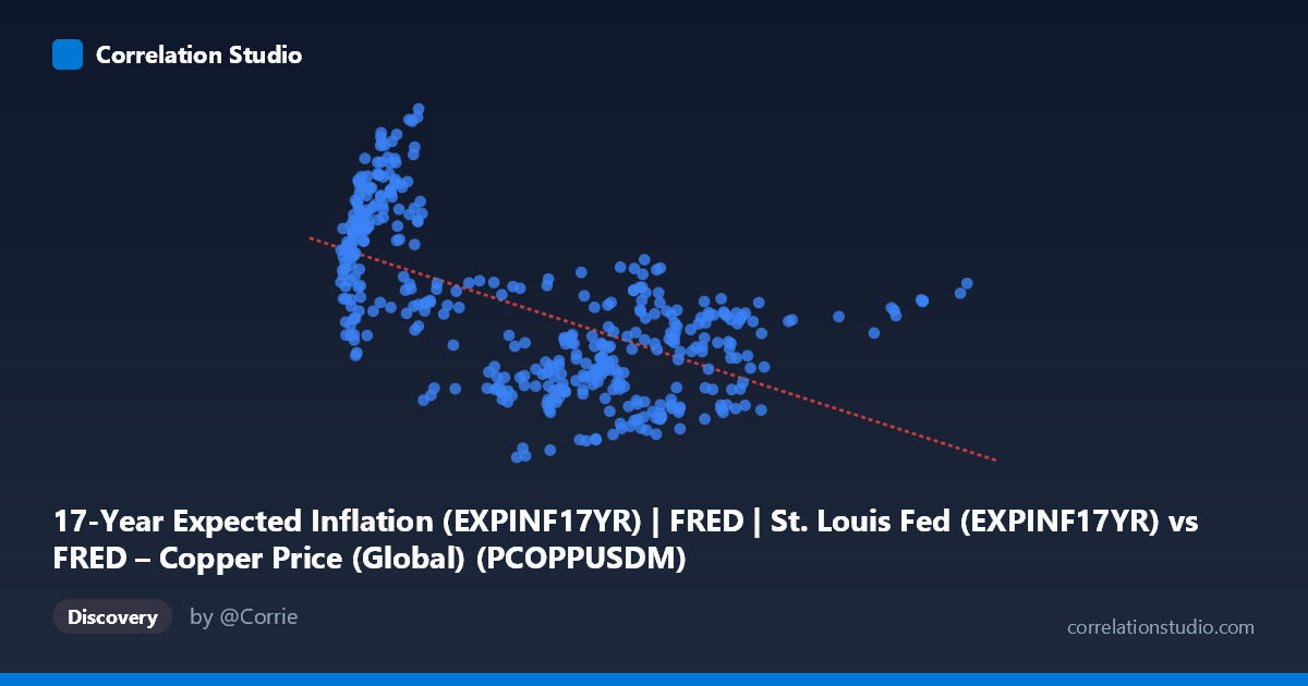
The scatterplot reveals a clear negative, moderately strong linear relationship between copper prices (X-axis) and 17-year expected inflation (Y-axis). As copper prices rise from roughly $1,400 to $13,000 per metric ton, expected long-term inflation tends to decline from around 3.5-3.75% down toward 1.4-2.0%. This is somewhat counterintuitive from a traditional economic standpoint, since copper is often viewed as an inflation hedge or leading indicator of economic activity that should correlate positively with inflation expectations.
2. Strength, Direction, and Statistical Confidence
The correlation coefficient of r = -0.64 indicates a moderate-to-strong negative relationship, with r² = 0.41 meaning copper prices statistically explain about 41% of the variance in inflation expectations — leaving the majority (59%) unexplained by this single variable. The 95% confidence interval [-0.69, -0.58] is tight and does not cross zero, and the p-value of ~0 confirms this relationship is highly statistically significant and not due to chance, given the large sample (n=411).
However, the Granger causality results are critical: neither variable significantly predicts the other in a temporal sense (X→Y: p=0.87; Y→X: p=0.996). This means despite the strong contemporaneous correlation, there is no evidence that past copper prices help forecast future inflation expectations, or vice versa. This strongly suggests the relationship is either driven by a third factor, is coincidental/structural (e.g., both trending due to macroeconomic regime shifts), or operates on a lag/frequency not captured by the tested lag structure.
3. Notable Patterns and Clusters
The data shows distinct clustering rather than a smooth continuous trend: - A low-copper/high-inflation cluster (X ≈ 1,600-3,300, Y ≈ 2.8-3.75) — likely representing an earlier era (possibly 1990s-2000s) with elevated long-term inflation expectations and lower copper prices. - A high-copper/low-to-moderate-inflation cluster (X ≈ 7,000-10,000, Y ≈ 1.6-2.5) — likely representing the 2010s-2020s commodity supercycle period with anchored inflation expectations. - A sparse, isolated high-X point (12,986, 2.38) that sits somewhat apart from the main cloud, worth checking as a potential leverage point.
The pattern looks less like a continuous causal curve and more like two temporal regimes with different mean inflation levels and different mean copper prices — consistent with the time coverage spanning 1992-2026.
4. Confounding Factors and Caveats
This is very likely a spurious or confounded regression driven by long-term trends (non-stationarity) rather than a genuine economic mechanism: - Both series may be trending over the 1992-2026 window due to independent macro regimes (e.g., the Great Moderation's declining inflation expectations coinciding with China-driven copper demand growth in the 2000s-2010s). - Monetary policy credibility (anchored inflation expectations since the 1990s) could be a common driver, causing 17-year inflation expectations to structurally decline over time regardless of copper. - Copper prices are influenced by global industrial demand, USD strength, and supply shocks — factors unrelated to long-run US inflation expectations. - The lack of Granger causality reinforces that this is likely a spurious correlation from shared time trends, not a functional/predictive relationship.
5. Suggested Further Investigation
- Detrend or difference both series (e.g., use year-over-year changes rather than levels) and re-run correlation/Granger tests to check if the relationship holds after removing long-term trend components. - Segment by decade/regime to test whether the correlation is driven entirely by the shift between the 1990s-2000s and 2010s-2020s periods rather than a consistent relationship. - Test rolling correlations over time to see if the r=-0.64 is stable or an artifact of pooling distinct macro eras. - Explore other explanatory variables (Fed funds rate, USD index, China PMI) that may better explain both series independently, indicating a common confounder rather than direct interaction.
X dataset: FRED – Copper Price (Global)
Y dataset: 17-Year Expected Inflation (EXPINF17YR) | FRED | St. Louis Fed
Part of experiment: Copper - FRED – Copper Price (Global) vs 17-Year Expected Inflation (EXPINF17YR) | FRED | St. Louis Fed