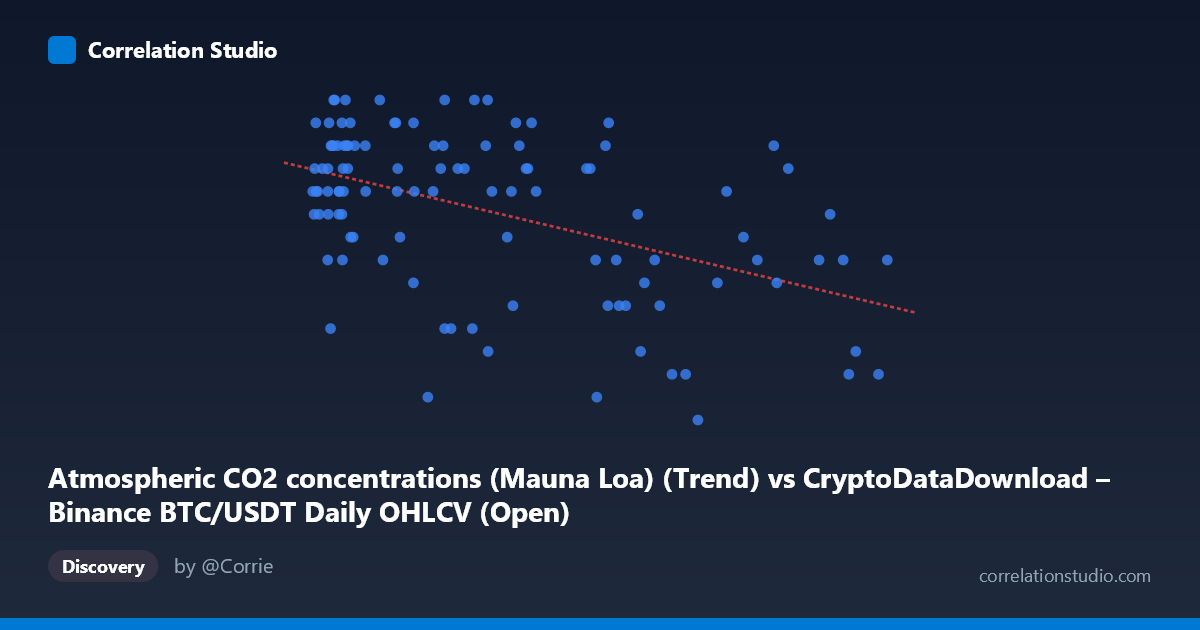
Atmospheric CO2 concentrations (Mauna Loa) (Trend) vs CryptoDataDownload – Binance BTC/USDT Daily OHLCV (Open)
- Pearson correlation (r)
- -0.4829
- Spearman correlation
- -0.3998
- p-value
- 0
- Sample size (n)
- 106
- 95% confidence interval
- -0.6168 to -0.3217
- Granger causality
- None
- Granger optimal lag
- 1
AI analysis
Analysis: BTC/USDT Price vs. Atmospheric CO2 Concentrations
1. What the Visualization Reveals
This scatterplot juxtaposes two datasets that have no plausible causal or mechanistic connection: Bitcoin's daily opening price (mislabeled in the axis metadata as CO2, but confirmed by column names to be BTC/USDT Open) and monthly mean atmospheric CO2 concentrations from Mauna Loa. The plot shows a moderate negative trend — as the X-axis variable increases, the Y-axis variable tends to decrease modestly — but the scatter is wide and noisy, with substantial vertical spread (Y ranging 17–31) at almost every X value, especially in the dense cluster below X=20,000.
2. Strength, Direction, and Statistical Meaning
The correlation coefficient (r = -0.458) indicates a moderate negative linear relationship, but r² = 0.210 means only about 21% of the variance in Y is explained by X — the remaining ~79% is driven by other factors entirely. The 95% confidence interval [-0.599, -0.289] excludes zero, and the p-value (1.3×10⁻⁶) is highly significant, so the correlation itself is statistically real and not a fluke of sampling — but "statistically significant" here should not be conflated with "practically meaningful" given the low r². Critically, the Granger causality tests show no significant predictive direction in either direction (X→Y p=0.94, Y→X p=0.69). This strongly suggests the correlation is not causal or even temporally predictive — it's more likely a spurious correlation arising from two independent trending time series (BTC price cycles and the steadily rising CO2 trend) that happen to move in opposite directions over the sampled window.
3. Notable Patterns and Outliers
The data shows a dense cluster of points at low X values (X < 20,000) with highly variable Y (17–31), suggesting this region carries little discriminating power despite containing half the sample. At higher X values (60,000), Y values trend more consistently lower (18–30 but skewing down), which drives the negative slope. Notable outliers include (58974, 18) and (114048.94, 19) — high X, low Y — and (35045, 31), (29233.2, 31) — mid-range X with high Y — that don't fit the trend well. No clear non-linear pattern (e.g., curvature) is obvious; the relationship looks like noisy linear decay at best.
4. Confounding Factors and Caveats
The core issue is a mismatched pairing of unrelated time series. Atmospheric CO2 rises in a smooth, near-monotonic secular trend independent of markets, while BTC price is driven by speculation, liquidity cycles, regulation, and macro sentiment. Any correlation here is almost certainly a time-trend artifact: both series may be drifting over the 2017–2026 window (CO2 rising steadily, BTC rising in bull/bear waves), and aligning them by date can produce apparent correlation without any real relationship. The failed Granger tests reinforce that neither series helps predict the other — a hallmark of spurious correlation between two autocorrelated trending series. Sample size (n=102 paired vs. N=816 population) and potential data resampling/alignment (monthly CO2 vs. daily BTC) may introduce additional aggregation artifacts.
5. Recommendations for Further Investigation
Rather than pursuing this pairing further, analysts should (a) detrend both series (e.g., first-difference or remove long-term trend components) and re-test correlation on the residuals to see if any relationship survives — it likely won't; (b) avoid using this correlation for any predictive or trading application, given the null Granger result and low r²; and (c) if investigating BTC price drivers, focus on economically plausible covariates (interest rates, on-chain metrics, exchange volume, regulatory news) rather than unrelated environmental series. This pairing is a good illustrative example of why correlation and significance testing alone are insufficient — causal plausibility and temporal predictive testing (like Granger causality) are essential guardrails against spurious conclusions.
X dataset: CryptoDataDownload – Binance BTC/USDT Daily OHLCV
Y dataset: Atmospheric CO2 concentrations (Mauna Loa)
Part of experiment: Bitcoin - CryptoDataDownload – Binance BTC/USDT Daily OHLCV vs Atmospheric CO2 concentrations (Mauna Loa)