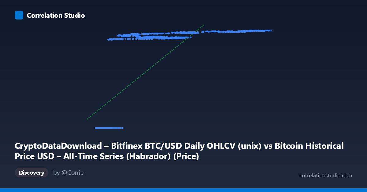
CryptoDataDownload – Bitfinex BTC/USD Daily OHLCV (unix) vs Bitcoin Historical Price USD – All-Time Series (Habrador) (Price)
- Pearson correlation (r)
- 0.7504
- Spearman correlation
- 0.9421
- p-value
- 0
- Sample size (n)
- 3902
- 95% confidence interval
- 0.7363 to 0.7638
- Granger causality
- None
- Granger optimal lag
- 10
- Time coverage
- 2015-02-09 to 2025-10-15
AI analysis
Analysis: Bitcoin Price (X) vs. Unix Timestamp (Y)
1. What the Visualization Reveals
This scatterplot is somewhat unusual in that the "Y" variable is actually a Unix timestamp (date), while "X" is the Bitcoin price in USD. Effectively, this plot shows price plotted against time, just with axes reversed from convention. What it reveals is Bitcoin's price trajectory across its history: long stretches of low prices (sub-$1,000) spanning many years, followed by increasingly volatile and higher-magnitude price excursions in later periods (2020–2025), including runs into the tens of thousands and eventually six-figure territory. The shape is not a clean linear trend — it looks more like a series of exponential "steps" or cycles, consistent with Bitcoin's well-known boom-bust halving cycles.
2. Strength, Direction, and Uncertainty
The Pearson correlation of r = 0.75 (r² = 0.563) indicates a moderately strong positive association — roughly 56% of the variance in the timestamp variable is "explained" by price (or vice versa). The narrow 95% CI [0.736, 0.764] and p-value of ~0 confirm this relationship is highly statistically reliable given the large sample (n=3,902) — there is essentially no doubt a positive association exists. However, statistical significance here reflects sample size and monotonic drift over time rather than a tight functional relationship; 44% of variance remains unexplained, which is substantial. Critically, the Granger causality tests show no significant predictive direction in either direction (X→Y: p=0.963; Y→X: p=0.812). This is actually expected and somewhat definitional: since Y is literally the timestamp, "causality" between calendar time and price isn't a meaningful causal question in the Granger sense — time doesn't "Granger-cause" price in a predictive-lag framework, and price doesn't cause time. This null result should be interpreted as a structural artifact of the variable choice, not a substantive finding about market dynamics.
3. Notable Patterns and Non-Linear Features
The data clearly show non-linear, cyclical clustering rather than a steady linear climb: - A dense cluster of low prices ($200–$1,500) persisting from 2015 through 2017, reflecting Bitcoin's early years. - A jump to the $4,000–$20,000 range through 2018–2020. - Explosive moves into the $30,000–$65,000 band during 2020–2022, with visible plateaus/consolidation (e.g., repeated values near $60,000 and $65,000 across different dates in 2024). - A further push toward $100,000–$125,000 in 2024–2025.
This staircase pattern — long consolidation plateaus punctuated by sharp vertical jumps — is classic of Bitcoin's boom/bust/halving cycle behavior and explains why a linear model only captures 56% of variance: log-linear or piecewise exponential growth would fit far better. The note that Spearman ρ exceeds Pearson r reinforces this — the relationship is monotonic but not linear, likely closer to exponential/logarithmic in true form.
4. Confounding Factors and Caveats
Several caveats apply: - Reversed causality framing: Since Y is a timestamp, this isn't really a "correlation between two market variables" — it's price vs. time, which will trivially trend positive as Bitcoin's price has grown over its history. The correlation coefficient here is more a measure of "how much has price risen over time" than a genuine bivariate relationship between independent phenomena. - Autocorrelation: Daily price data is highly autocorrelated (today's price depends on yesterday's), which inflates apparent statistical significance and violates independence assumptions underlying p-values. - Non-stationarity: Bitcoin price is a non-stationary series with structural breaks (halvings, regulatory events, exchange collapses), making simple linear correlation a poor summary metric. - Survivorship/exchange-specific bias: Bitfinex-specific OHLCV may reflect exchange-specific liquidity events not representative of the broader market.
5. Actionable Insights
- Refit with a non-linear model: Given the Spearman/Pearson divergence and visual staircase pattern, a log-linear (log(price) vs. time) or exponential regression would likely explain substantially more variance than the current 56%. - Segment by halving cycle: Analyzing sub-periods (2015–2017, 2017–2020, 2020–2022, 2022–2025) separately may reveal more consistent, higher-r relationships within each cycle. - Avoid causal interpretation: Since one axis is literally time, do not over-interpret the Granger causality null result as evidence about market efficiency — it's a mechanical consequence of the variable setup. If the intent was to test Bitfinex price vs. some other market indicator, verify that the Y column was correctly specified rather than accidentally set to timestamp. - Volatility modeling: Given the clear heteroskedasticity (variance increasing with price level), consider log-transforming price before further statistical modeling (e.g., GARCH-style volatility analysis) to better capture cycle-dependent risk.
X dataset: Bitcoin Historical Price USD – All-Time Series (Habrador)
Y dataset: CryptoDataDownload – Bitfinex BTC/USD Daily OHLCV
Part of experiment: Bitcoin - Bitcoin Historical Price USD – All-Time Series (Habrador) vs CryptoDataDownload – Bitfinex BTC/USD Daily OHLCV