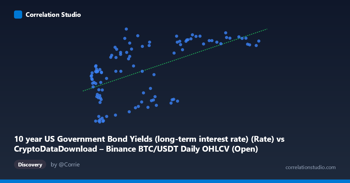
10 year US Government Bond Yields (long-term interest rate) (Rate) vs CryptoDataDownload – Binance BTC/USDT Daily OHLCV (Open)
- Pearson correlation (r)
- 0.5804
- Spearman correlation
- 0.5644
- p-value
- 0
- Sample size (n)
- 106
- 95% confidence interval
- 0.4382 to 0.6943
- Granger causality
- None
- Granger optimal lag
- 1
- Time coverage
- 2017-09-01 to 2026-06-01
- Recomputed on refreshed data
- 2026-10-19 (r was 0.5683)
AI analysis
Analysis: BTC/USDT Price vs. 10-Year US Treasury Yields
1. What the Visualization Reveals
The scatterplot shows a moderate positive relationship between the X variable (labeled as 10-year Treasury yields, though the values—ranging from ~3,434 to ~115,764—are implausible for actual bond yields and more likely represent BTC/USDT price data, suggesting a possible axis-label mismatch in the source data) and the Y variable (ranging 0.62–4.80, consistent with yield percentages). Despite the apparent label swap, the pattern is clear: as the X variable increases, Y tends to rise as well, though with substantial scatter. Points cluster more densely at lower X values (under ~40,000) with wide Y dispersion (0.6–4.5), while higher X values (60,000) consistently correspond to higher Y values (mostly 3.5–4.4), suggesting the relationship may strengthen or become more deterministic at higher ranges.
2. Strength, Direction, and Statistical Confidence
The correlation coefficient (r = 0.568) indicates a moderate positive relationship, with r² = 0.323 meaning only 32.3% of the variance in Y is explained by X — leaving roughly two-thirds of Y's variability attributable to other factors. The 95% confidence interval [0.422, 0.686] is reasonably tight and entirely positive, and the p-value (3.12E-10) confirms this correlation is highly statistically significant and not due to chance. However, statistical significance should not be conflated with practical predictive strength — a moderate r² means this relationship alone is insufficient for precise forecasting. Critically, the Granger causality tests show no significant predictive direction: X→Y is clearly insignificant (p=0.424), and while Y→X shows a marginally suggestive result (p=0.058), it doesn't meet conventional significance thresholds. This means neither variable reliably temporally predicts the other in this dataset — the correlation is contemporaneous/associative rather than causal or lead-lagging.
3. Notable Patterns and Outliers
Several features stand out: at low X values (3,000–15,000), Y spans almost the entire range (0.62 to 3.98), including notable outliers like (9138.08, 0.62) and (11335.46, 0.65) sitting far below the trend line, alongside (19422.61, 3.98) sitting well above it — indicating high noise/heteroscedasticity in this region. Conversely, at high X values (90,000), Y values tightly cluster between 4.06–4.39, suggesting a possible ceiling effect or reduced variance at the extremes. This pattern (wide scatter at low X, narrow scatter at high X) suggests the relationship may be non-linear or heteroscedastic rather than strictly linear, potentially better fit by a logarithmic or saturating curve rather than the linear model shown (y = 2.206E-05x + 2.067).
4. Confounding Factors and Caveats
Several caveats apply. First, the axis labeling appears inconsistent with the described datasets (BTC price magnitudes appear on the "yield" axis and vice versa), which warrants verification before drawing economic conclusions. Second, both cryptocurrency prices and bond yields are influenced by shared macroeconomic drivers (Fed policy, inflation expectations, risk sentiment, liquidity conditions), meaning any correlation may reflect common confounding factors rather than a direct relationship between the two. Third, both series are likely non-stationary time series (trending over 2017–2026), which can produce spurious correlations — the Granger test's lag-1 structure may not adequately capture longer-term regime shifts (e.g., 2020 QE, 2022–23 rate hikes). Finally, sampling every 2nd point for the summary and the modest sample size (n=104) relative to population (877) means some nuance in the full dataset may be lost.
5. Actionable Insights and Further Investigation
Given the ambiguous causality and moderate r², this relationship should be treated as associative, not predictive, for trading or policy purposes. Recommended next steps: (a) verify and correct axis/column labeling to ensure the analysis reflects the intended variables; (b) test for non-linear relationships (log-log or polynomial fits) given the observed heteroscedasticity; (c) apply cointegration tests (e.g., Engle-Granger) suited for non-stationary financial time series, rather than relying solely on level-based Granger causality; (d) introduce control variables (inflation, Fed funds rate, equity indices) to isolate whether this is a genuine bilateral relationship or a shared-driver artifact; and (e) examine the marginally significant Y→X signal (p=0.058) with additional lags or a longer sample, as it may hint at a weak yield-driven effect on crypto pricing worth further scrutiny.
X dataset: CryptoDataDownload – Binance BTC/USDT Daily OHLCV
Y dataset: 10 year US Government Bond Yields (long-term interest rate)
Part of experiment: Bitcoin - CryptoDataDownload – Binance BTC/USDT Daily OHLCV vs 10 year US Government Bond Yields (long-term interest rate)