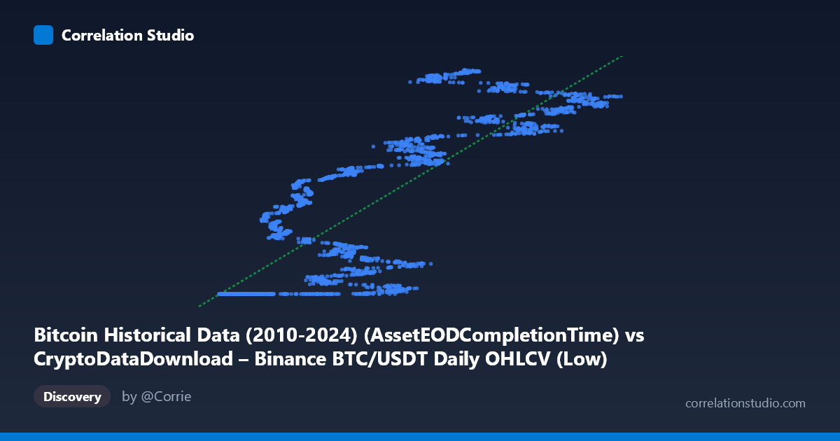
Bitcoin Historical Data (2010-2024) (AssetEODCompletionTime) vs CryptoDataDownload – Binance BTC/USDT Daily OHLCV (Low)
- Pearson correlation (r)
- 0.8546
- Spearman correlation
- 0.89
- p-value
- 0
- Sample size (n)
- 3191
- 95% confidence interval
- 0.845 to 0.8637
- Granger causality
- None
- Granger optimal lag
- 10
- Time coverage
- 2017-08-17 to 2026-05-20
AI analysis
Analysis: Bitcoin Timestamp vs. BTC/USDT Low Price
1. What the Visualization Reveals
This scatterplot is somewhat unusual in that the "X" variable is actually a timestamp/completion-time field rather than a conventional independent variable, and Y is the daily low price of BTC/USDT. Despite the mismatched labeling, the effective relationship being plotted is time progression vs. Bitcoin price. The data shows a clear upward-sloping pattern, consistent with Bitcoin's well-documented long-term price appreciation from 2017 to 2026. Notably, a large cluster of points sits near the minimum X values with Y compressed tightly around ~1,614,337,000 — this looks like an artifact (possibly repeated/placeholder timestamps or an early low-volatility price regime) rather than genuine dispersion.
2. Strength, Direction, and Statistical Confidence
The correlation coefficient (r = 0.855) indicates a strong positive relationship, with r² = 0.730 meaning roughly 73% of the variance in Y (price) is explained by X (time). The remaining ~27% reflects price volatility, cyclical bull/bear swings, and short-term noise not captured by a simple linear time trend. The 95% CI [0.845, 0.864] is narrow, and p ≈ 0 confirms this correlation is highly statistically significant and not due to chance, aided by the large sample size (n = 3,191). However, the Granger causality tests show no significant predictive direction in either direction (X→Y: p=0.35; Y→X: p=0.19). This is an important caveat: strong correlation here reflects a shared long-term trend (time-based drift), not a dynamic lead-lag forecasting relationship — X does not "Granger-cause" Y or vice versa in a way useful for short-term prediction.
3. Notable Patterns and Outliers
The most striking feature is the dense cluster at low X values (~3,000–20,000) with Y pinned near 1,614,337,000 — a near-constant value suggesting these are early/flat entries, sentinel values, or a data-quality issue (e.g., unfilled OHLCV rows defaulting to a fixed low). Beyond this cluster, the relationship becomes visibly non-linear: price growth accelerates in stages (e.g., jumps between the 1.61B and 1.78B range) rather than following a smooth line, consistent with Bitcoin's actual history of sharp bull runs (2020-21, 2023-24) punctuated by consolidation/crash periods. The linear regression (y = 1459.11x + 1.61E9) is a rough approximation; residuals likely show heteroskedasticity, with wider scatter at higher X (more recent times, higher volatility/price levels).
4. Confounding Factors and Caveats
Several caveats apply: - Variable mislabeling/units: X is labeled as a timestamp field ("AssetEODCompletionTime"), not a substantive market variable — this is essentially a time-series trend, not a causal economic relationship between two independent phenomena. - Autocorrelation: Both time and price are highly autocorrelated series; standard Pearson r/p-values assume independent observations, which is violated here, likely inflating apparent significance. - Non-stationarity: Bitcoin prices are non-stationary (trending, regime-dependent), which can produce spurious correlation with any monotonic trend variable, including time itself. - Data artifacts: The flat cluster at Y≈1.614B for varying X suggests placeholder/missing data that should be cleaned before drawing conclusions.
5. Suggested Next Steps
1. Clarify the X variable — confirm whether it's meant to be a proxy for calendar time or something else; if it's truly time, treat this as a time-series trend analysis rather than a bivariate correlation study. 2. Clean the flat-value cluster at Y≈1.614337B to check if it's a data-entry artifact skewing both r and the regression. 3. Use time-series-appropriate methods (e.g., differencing, cointegration tests, ARIMA) instead of Pearson correlation, given autocorrelation and non-stationarity concerns. 4. Segment by market regime (bull/bear cycles) to see if the relationship holds consistently or is driven by a few large trend segments. 5. Given the null Granger causality result, do not use this relationship for predictive trading models — it reflects historical trend alignment, not a forecastable lead-lag dynamic.
X dataset: CryptoDataDownload – Binance BTC/USDT Daily OHLCV
Y dataset: Bitcoin Historical Data (2010-2024)
Part of experiment: Bitcoin - CryptoDataDownload – Binance BTC/USDT Daily OHLCV vs Bitcoin Historical Data (2010-2024)