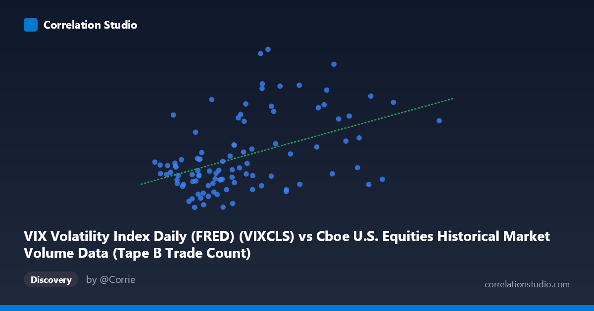
VIX Volatility Index Daily (FRED) (VIXCLS) vs Cboe U.S. Equities Historical Market Volume Data (Tape B Trade Count)
- Pearson correlation (r)
- 0.4515
- Spearman correlation
- 0.3974
- p-value
- 0.000003
- Sample size (n)
- 99
- 95% confidence interval
- 0.2789 to 0.5958
- Granger causality
- None
- Granger optimal lag
- 1
AI analysis
Analysis: VIX Volatility Index vs. Cboe Tape B Trade Count
1. Overall Relationship The scatterplot reveals a moderate positive relationship between the VIX Volatility Index and Cboe U.S. Equities Tape B Trade Count. As VIX values rise — indicating heightened market fear and implied volatility — the number of Tape B trades tends to increase. The linear regression equation (y = 7.105×10⁻⁶x + 12.64) confirms this upward slope, which is economically intuitive: periods of elevated market anxiety typically drive greater retail and institutional trading activity across the smaller-cap and ETF-heavy securities captured in Tape B. However, the scatter is wide, suggesting the relationship is far from deterministic.
2. Correlation Strength, Direction, and Causality The Pearson correlation of r = 0.4515 indicates a moderate positive association, but the coefficient of determination (R² = 0.2038) is the more sobering metric — only ~20.4% of the variance in Tape B trade count is explained by VIX levels. The remaining ~79.6% is driven by other factors entirely outside this model. The 95% confidence interval for r spans [0.279, 0.596], confirming the effect is real but meaningfully uncertain in its precise magnitude. The p-value of 2.73×10⁻⁶ firmly rejects the null hypothesis of zero correlation, so the statistical significance is not in question for this sample. Critically, however, the Granger causality tests are entirely non-significant in both directions (X→Y: F=0.0006, p=0.980; Y→X: F=0.0004, p=0.984), meaning that neither variable temporally predicts the other with a one-period lag. The correlation reflects a contemporaneous co-movement rather than any leadâ€"lag predictive relationship — knowing yesterday's VIX does not help forecast today's trade count, and vice versa.
3. Notable Patterns, Clusters, and Outliers Several features stand out visually. The bulk of observations cluster in the VIX range of ~700K–1.1M (noting the X-axis represents the raw FRED series value in its native units) with Y values between roughly 15–22, forming a dense core. Above approximately X = 1.2M, the data becomes sparser but more dispersed, with several high-Y outliers including notably (1,115,472 / 31.05), (1,085,027 / 30.61), and (1,092,250 / 27.44) that sit well above the regression line. There are also puzzling low-Y observations at high X values — for instance, (1,808,757 / 23.57) and (1,578,717 / 17.44) — suggesting some extreme VIX readings did not produce elevated trade counts, which could reflect thin trading days or data anomalies. A potential non-linear pattern is hinted at: the relationship may follow more of a threshold or exponential curve, where trade counts accelerate only beyond certain VIX stress levels rather than increasing uniformly.
4. Confounding Factors and Caveats Several important caveats apply. First, Tape B specifically covers NYSE American and regional exchange listings (smaller-cap stocks and ETFs), meaning its trade count is influenced by factors specific to that segment — ETF arbitrage mechanics, retail participation platforms, and market-maker obligations — that are only loosely connected to broad VIX dynamics. Second, secular trends in electronic trading volumes over the January–May 2026 window could create spurious correlation if both series share a common time trend; neither variable was explicitly detrended in this analysis. Third, the population size (N=1,980) versus sample size (n=99) gap means roughly 95% of data points are not represented here, and the sample's representativeness is unverified. Fourth, VIX itself is a forward-looking implied volatility measure derived from S&P 500 options, introducing a conceptual mismatch with realized equity market microstructure activity. Finally, market structure events — such as exchange outages, earnings seasons, or options expiration dates — could drive correlated spikes in both series simultaneously without any causal link.
5. Actionable Insights and Further Investigation Practitioners should not use lagged VIX as a standalone predictor for Tape B trade volume, given the failed Granger tests. However, the contemporaneous correlation is strong enough to be useful in real-time risk dashboards or intraday liquidity models where same-period VIX readings are available. To improve the model, analysts should: (1) test non-linear specifications (log-log or spline regression) given the apparent curvature in the upper tail; (2) include additional covariates such as overall market volume (Tape A/C), S&P 500 realized volatility, and day-of-week effects to increase explanatory power beyond the current 20%; (3) investigate the outlier cluster near VIX ~1.09–1.13M with anomalously high trade counts, as these may represent identifiable market events worth understanding; and (4) extend the time window beyond five months to test whether this relationship is stable across different volatility regimes, particularly full market cycles spanning both crisis and calm periods.
X dataset: Cboe U.S. Equities Historical Market Volume Data
Y dataset: VIX Volatility Index Daily (FRED)
Part of experiment: Daily - Cboe U.S. Equities Historical Market Volume Data vs VIX Volatility Index Daily (FRED)