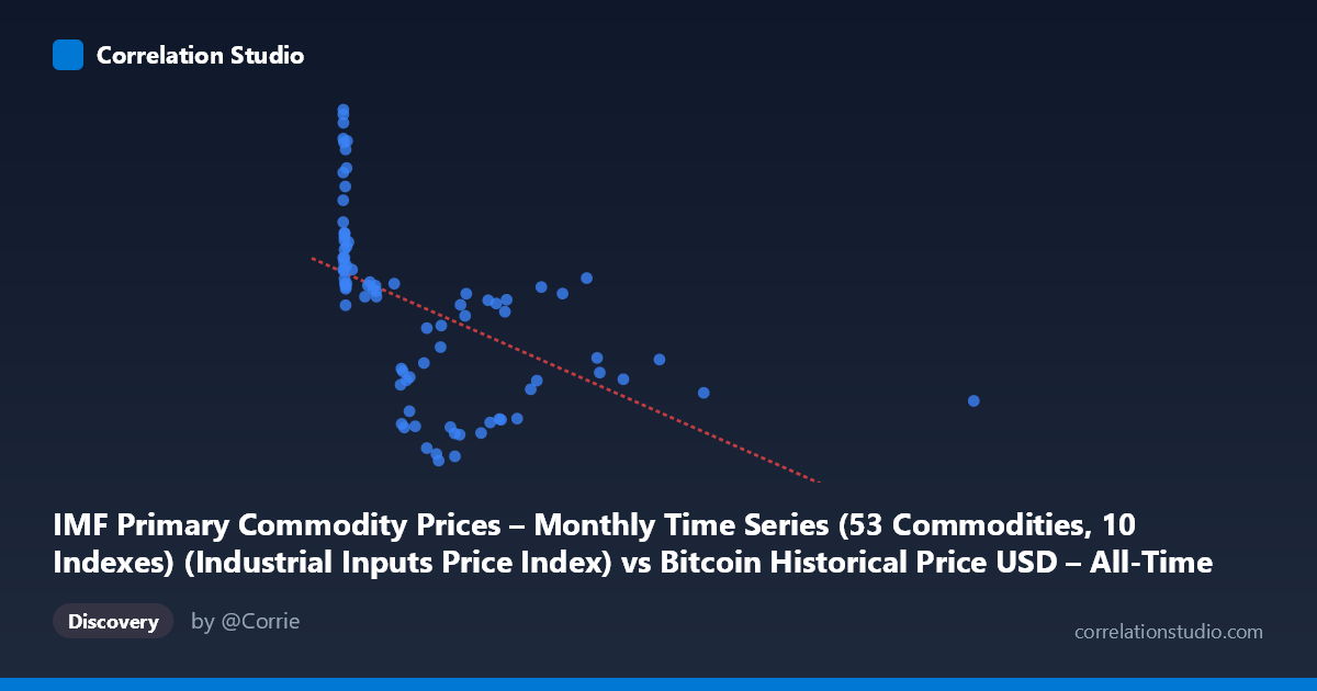
IMF Primary Commodity Prices – Monthly Time Series (53 Commodities, 10 Indexes) (Industrial Inputs Price Index) vs Bitcoin Historical Price USD – All-Time Series (Habrador) (Price)
- Pearson correlation (r)
- -0.5156
- Spearman correlation
- -0.7451
- p-value
- 0.000001
- Sample size (n)
- 83
- 95% confidence interval
- -0.6581 to -0.3374
- Granger causality
- None
- Granger optimal lag
- 1
AI analysis
Analysis: Bitcoin Price vs. Industrial Inputs Price Index
1. Relationship Overview
The scatterplot reveals a moderate negative relationship between the IMF Industrial Inputs Price Index (X) and Bitcoin's historical USD price (Y). Note the axis labeling is reversed from convention here—X represents the commodity index, Y represents Bitcoin price. The data shows a clear pattern: at low index values (X < 50), Bitcoin prices cluster in a wide band (roughly 155–217), while as the index rises above 200, Bitcoin prices settle into a narrower, lower band (105–160). This is not a simple linear cloud but resembles a decaying curve — high Y-variance at low X, compressing as X increases.
2. Strength, Direction, and Statistical Confidence
The Pearson correlation (r = -0.516, R² = 0.266) indicates a moderate negative linear association, with the industrial inputs index explaining about 27% of the variance in Bitcoin price — leaving 73% unexplained by this single variable. The 95% CI [-0.658, -0.337] is comfortably away from zero, and the p-value (6.1×10⁻⁷) confirms this correlation is highly unlikely due to chance. However, statistical significance should not be conflated with practical predictive power — R² of 0.27 means this relationship alone is a weak-to-moderate predictor at best.
Critically, the Granger causality tests show no significant predictive direction in either direction (X→Y: p=0.399; Y→X: p=0.692). This means neither variable's past values help forecast the other's future values at a 1-period lag. This strongly suggests the correlation is not causal in a temporal/mechanistic sense — it likely reflects a shared underlying driver (e.g., both responding to global macroeconomic cycles, USD strength, or risk sentiment) rather than one variable leading the other.
3. Notable Patterns and Outliers
Several structural features stand out: - Dense low-X cluster: The majority of points sit at X < 50, spanning nearly the full Y range (105–217) — including extreme high-Y outliers (e.g., Y=217.07, 215.54, 212.91 at X near 0). These early-Bitcoin-era points likely correspond to a specific historical period (possibly 2017 bull run or early data collection) and disproportionately anchor the "low-X, high-Y" pattern. - High-X tail: Very few points exist beyond X=1000 (5 points up to X=2452), and these consistently show mid-range, compressed Y values (124–164) — this sparse tail has outsized leverage on the regression slope. - Non-linearity signal: The note that Spearman ρ exceeds Pearson r indicates the relationship is better described as monotonic-but-curved rather than strictly linear — consistent with a log-decay or power-law shape, common when comparing a price index against a highly volatile asset like Bitcoin.
4. Confounding Factors and Caveats
Several caveats limit causal interpretation: - Time-series confound: Both series are macro/financial time series (2010–2017) that may share a common trend, seasonality, or third-factor influence (e.g., global growth, dollar index, monetary policy) rather than being directly linked. - Reversed/mismatched axis metadata: The dataset descriptions are inconsistent (X described as Bitcoin, Y described as commodity index) — this warrants confirmation of what's actually plotted to avoid misinterpretation. - Sparse high-X leverage: With only a handful of points driving the tail behavior, outliers could substantially distort both the correlation coefficient and regression slope. - N vs n mismatch: Only 83 of 449 available population points were sampled, so this correlation may not fully represent the entire dataset, especially given monthly time-series autocorrelation (adjacent months aren't independent observations, inflating apparent significance).
5. Suggested Next Steps
1. Verify variable labeling — confirm which axis is Bitcoin price vs. commodity index before drawing economic conclusions. 2. Fit non-linear models (log-linear, polynomial) given the Spearman/Pearson divergence — a log transform of X or Y may substantially improve fit. 3. Segment by time period — plot with a color gradient by date to check if the relationship is driven by a specific era (e.g., 2011 vs. 2017) rather than being stable throughout. 4. Test with more lags in Granger causality (beyond lag=1) and consider cointegration analysis, since both series are non-stationary price trends. 5. Control for common macro factors (USD index, equity markets, inflation expectations) using multivariate regression to isolate any genuine bilateral relationship from shared confounds.
X dataset: Bitcoin Historical Price USD – All-Time Series (Habrador)
Y dataset: IMF Primary Commodity Prices – Monthly Time Series (53 Commodities, 10 Indexes)
Part of experiment: Bitcoin - Bitcoin Historical Price USD – All-Time Series (Habrador) vs IMF Primary Commodity Prices – Monthly Time Series (53 Commodities, 10 Indexes)