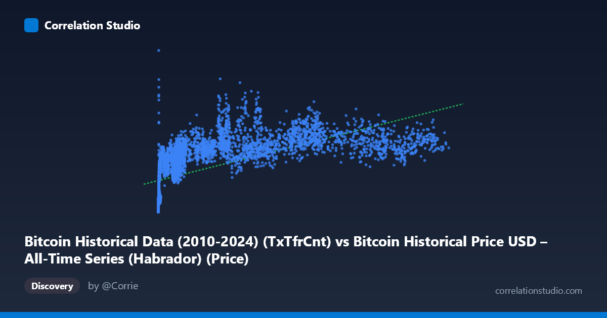
Bitcoin Historical Data (2010-2024) (TxTfrCnt) vs Bitcoin Historical Price USD – All-Time Series (Habrador) (Price)
- Pearson correlation (r)
- 0.6289
- Spearman correlation
- 0.903
- p-value
- 0
- Sample size (n)
- 5764
- 95% confidence interval
- 0.6131 to 0.6443
- Granger causality
- None
- Granger optimal lag
- 10
AI analysis
Analysis: Bitcoin Transaction Count (TxTfrCnt) vs. Price (USD)
1. Relationship Overview
The scatterplot shows a moderate positive relationship between Bitcoin's daily transaction/transfer count and its USD price, but the relationship is clearly non-linear. At low transaction counts (roughly 0–1,000), prices span an enormous range — from under $1,000 to over $600,000 — indicating that in Bitcoin's early years, price often rose independently of transaction volume, likely driven by speculative adoption rather than network usage. As transaction counts climb into the tens of thousands, price growth continues but with diminishing marginal sensitivity, producing a concave, logarithmic-like curve rather than a straight line.
2. Strength, Direction, and Uncertainty
The Pearson correlation (r = 0.629) indicates a moderate positive linear association, with r² = 0.396 meaning only ~40% of the variance in price is explained by transaction count under a linear model — the majority of price variance is driven by other factors. The 95% CI [0.613, 0.644] is tight and the p-value is effectively 0, so we can be highly confident a real, non-zero linear association exists — but confidence in the existence of a relationship is not the same as confidence in linear predictive power, which remains modest. The note that Spearman ρ exceeds Pearson r reinforces that a monotonic, non-linear model (log or polynomial) would fit the data meaningfully better. Critically, Granger causality tests found no significant predictive direction either way (X→Y: p = 0.974; Y→X: p = 0.459) at 10 lags — meaning transaction count does not reliably lead price, nor does price lead transaction count, in a time-series forecasting sense. This is an important caveat: cross-sectional correlation exists, but it does not translate into temporal predictability.
3. Patterns, Clusters, and Outliers
The data shows a clear fan/wedge shape: tight clustering at low X values with wide price dispersion, narrowing somewhat as X increases (though scatter remains high even at high transaction counts — e.g., points near X≈45,000–65,000 span prices from ~$780K to ~$1.3M). Several points stand out as behaviorally distinct: extremely low X (X < 1) with prices in the hundreds to low thousands represent Bitcoin's earliest genesis-era data, while high-X, moderate-price points (e.g., X≈120,000, Y≈806,000) suggest periods of high network activity without proportional price gains — possibly congestion or bear-market usage. This pattern is consistent with several distinct market regimes/cycles (bull runs, crashes, adoption phases) rather than one continuous relationship.
4. Confounders and Caveats
This is time-series data spanning 2010–2026, so both variables are likely non-stationary and trending upward over time (network growth and price appreciation both correlate with the passage of time and broader adoption). This raises the risk of spurious correlation via a shared trend — a classic confound in financial/time-series analysis. Other unmodeled factors — macroeconomic conditions, regulatory news, exchange volume, halving cycles, speculative sentiment, and institutional adoption — almost certainly drive price more directly than raw transfer counts. Additionally, transaction count can be inflated by non-economic activity (e.g., spam transactions, batching changes, or protocol-level shifts like SegWit/Lightning adoption), decoupling it from genuine economic signal.
5. Suggestions for Further Investigation
Given the Spearman/Pearson discrepancy, refitting with a log-log or log-linear model (log(price) ~ log(transactions) or log(transactions)) should substantially improve fit and better reflect Bitcoin's exponential growth dynamics. Detrending both series (e.g., differencing, or using log-returns) before re-running correlation and Granger tests would help distinguish genuine relationship from shared temporal trend — this is standard practice for cointegrated financial series. It would also be valuable to segment analysis by market cycle/halving era to check whether the X-Y relationship is regime-dependent, and to incorporate additional covariates (active addresses, exchange volume, hash rate) in a multivariate model to better isolate transaction count's true marginal contribution to price.
X dataset: Bitcoin Historical Price USD – All-Time Series (Habrador)
Y dataset: Bitcoin Historical Data (2010-2024)
Part of experiment: Bitcoin - Bitcoin Historical Price USD – All-Time Series (Habrador) vs Bitcoin Historical Data (2010-2024)