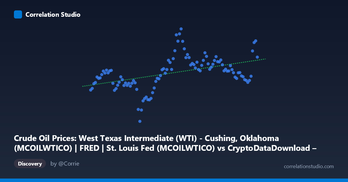
Crude Oil Prices: West Texas Intermediate (WTI) - Cushing, Oklahoma (MCOILWTICO) | FRED | St. Louis Fed (MCOILWTICO) vs CryptoDataDownload – Binance BTC/USDT Daily OHLCV (Unix)
- Pearson correlation (r)
- 0.4496
- Spearman correlation
- 0.5188
- p-value
- 0.000001
- Sample size (n)
- 106
- 95% confidence interval
- 0.2831 to 0.5898
- Granger causality
- None
- Granger optimal lag
- 8
AI analysis
Analysis: WTI Crude Oil Prices vs. Time (Mislabeled Axes)
Important note on data labeling: The axis labels appear swapped or mismatched — the X-axis is described as WTI crude oil prices but contains Unix timestamps (values in the 1.5–1.78 trillion range, i.e., dates from 2017–2026), while Y-axis values (16–115) look like actual WTI price levels in USD/barrel. This analysis treats X as time and Y as WTI crude oil price, which is consistent with the data structure.
1. What the Visualization Reveals The scatterplot shows WTI crude oil prices plotted across roughly a nine-year span (2017–2026). The data reveals a moderate upward drift in price over time, punctuated by significant volatility — including a sharp trough near mid-2020 (Y=16.55, coinciding with the COVID-19 demand collapse) and a peak near 2022 (Y=109.55, consistent with post-pandemic recovery and the Russia-Ukraine energy shock). Rather than a clean linear trend, the chart shows a noisy, cyclical pattern with multiple local peaks and troughs layered on top of a gentle long-term rise.
2. Strength and Direction of the Correlation The correlation coefficient (r = 0.45) indicates a moderate positive relationship between time and oil price. However, r² = 0.203 means only about 20% of the variance in oil prices is explained by the linear time trend — the remaining 80% is driven by other factors (supply shocks, geopolitical events, demand cycles, etc.). The 95% CI [0.284, 0.590] is reasonably tight and excludes zero, and the p-value (1.29E-06) confirms this relationship is highly statistically significant — unlikely to be due to chance. That said, statistical significance with modest r² tells us the trend is real but weak as a predictive tool. The Granger causality tests show no significant predictive direction in either direction (X→Y: p=0.071; Y→X: p=0.222), meaning time itself doesn't "cause" price in any dynamic forecasting sense — unsurprising, since time is not a causal driver but a scaffold on which other economic forces act.
3. Notable Patterns and Outliers Several features stand out: (a) a pronounced trough around 2020 (Y=16.55, 39.63, 39.40) reflecting the pandemic oil price crash and even negative-price events in WTI futures that year; (b) a peak cluster around 2022 (Y=109.55, 84.26–89.43) tied to the Ukraine war energy crisis; (c) a recent resurgence toward 2025–2026 with values climbing back into the 70–102 range, suggesting renewed upward momentum. The relationship is clearly non-linear/cyclical rather than a steady linear climb — a simple regression line understates the boom-bust structure evident in the scatter.
4. Confounding Factors and Caveats Oil prices are influenced by numerous confounders not captured by a simple time trend: OPEC+ production decisions, US shale output, global recessions, currency (USD) strength, geopolitical conflicts, and inventory levels. Using "time" as a predictor is really a proxy for an accumulation of these unmeasured, non-stationary macro factors. Additionally, since both series likely have trends/autocorrelation, the correlation may partly reflect spurious trend correlation rather than genuine mechanistic linkage — a common risk in time-series correlations lacking cointegration testing.
5. Actionable Insights Given the weak Granger causality and modest r², a linear time-trend model is not suitable for forecasting oil prices. Better approaches would include: (1) decomposing the series into trend/cycle/seasonal components (e.g., STL decomposition) to isolate structural cycles like the 2020 crash and 2022 spike; (2) testing cointegration with actual economic drivers (USD index, OPEC output, inventories) instead of raw time; and (3) using ARIMA/GARCH models suited to oil's volatility clustering rather than OLS regression. Analysts should treat this correlation as descriptive context (oil trended upward with high volatility over the period) rather than a predictive relationship.
X dataset: CryptoDataDownload – Binance BTC/USDT Daily OHLCV
Y dataset: Crude Oil Prices: West Texas Intermediate (WTI) - Cushing, Oklahoma (MCOILWTICO) | FRED | St. Louis Fed
Part of experiment: Bitcoin - CryptoDataDownload – Binance BTC/USDT Daily OHLCV vs Crude Oil Prices: West Texas Intermediate (WTI) - Cushing, Oklahoma (MCOILWTICO) | FRED | St. Louis Fed