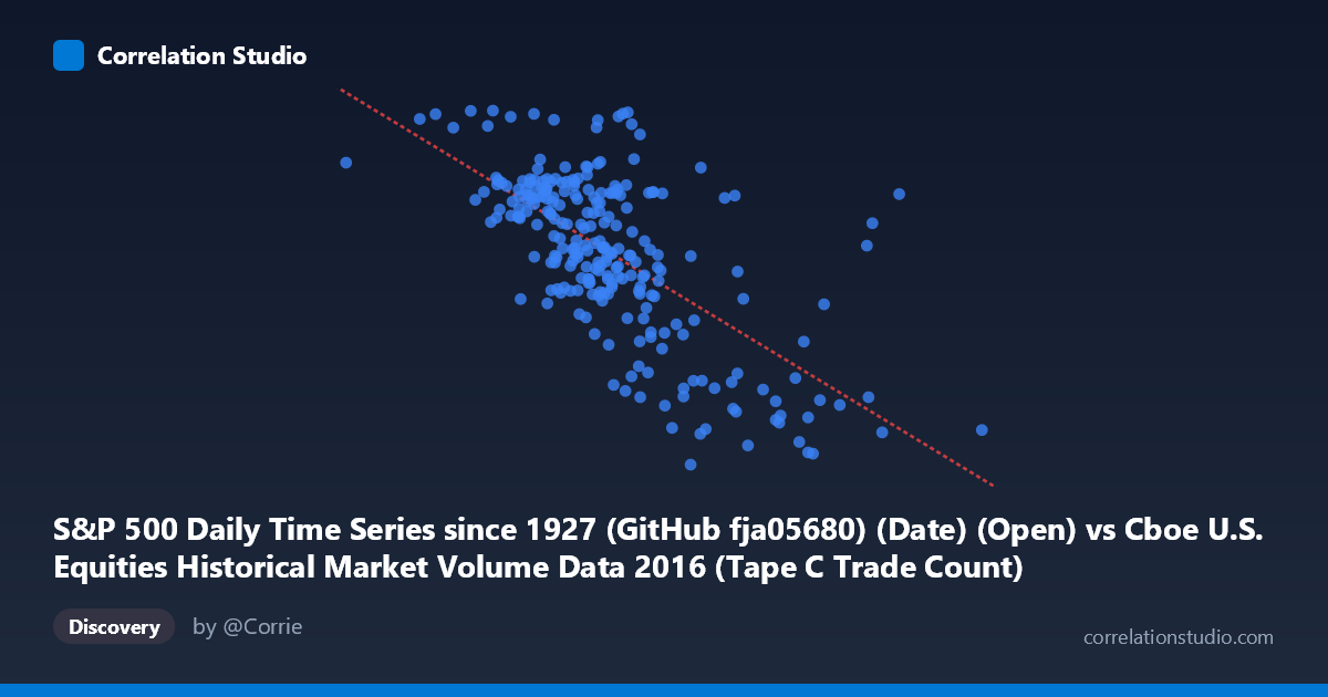
S&P 500 Daily Time Series since 1927 (GitHub fja05680) (Date) (Open) vs Cboe U.S. Equities Historical Market Volume Data 2016 (Tape C Trade Count)
- Pearson correlation (r)
- -0.66
- Spearman correlation
- -0.6144
- p-value
- 0
- Sample size (n)
- 252
- 95% confidence interval
- -0.7244 to -0.584
- Granger causality
- None
- Granger optimal lag
- 1
AI analysis
Analysis: S&P 500 Opening Price vs. Cboe Tape C Trade Count (2016)
Relationship Overview The scatterplot reveals a moderately strong negative relationship between the S&P 500 daily opening price and the Cboe Tape C trade count throughout 2016. As the S&P 500 opened at higher price levels, the number of trades recorded under Tape C (NYSE Arca-listed securities) tended to decline. The linear regression equation (y = −0.000456x + 2,419.53) captures this downward slope, suggesting that for every 100,000-point increase in the opening price index value, trade count decreases by roughly 45.6 units. The data spans a full calendar year (January–December 2016), with 252 paired observations drawn from a population of 3,622 records, providing a reasonably representative daily snapshot of market activity.
Correlation Strength and Statistical Significance The Pearson correlation of r = −0.660 indicates a moderate-to-strong inverse association, and the R² of 0.4355 means that approximately 43.6% of the variance in Tape C trade counts is explained by the S&P 500 opening price level alone — a meaningful but incomplete explanation, leaving over 56% attributable to other factors. The 95% confidence interval of [−0.724, −0.584] is relatively narrow and does not cross zero, reinforcing the reliability of this negative direction. The p-value of effectively zero confirms this is highly unlikely to be a chance finding. However, the Granger causality tests complicate interpretation significantly: neither direction (X→Y nor Y→X) achieves statistical significance (F = 0.28, p = 0.60 for X→Y; F = 0.20, p = 0.65 for Y→X at lag 1). This means that while a strong contemporaneous correlation exists, neither variable demonstrably predicts the other temporally — the relationship is associative rather than directionally causal on a day-to-day lag basis.
Notable Patterns, Clusters, and Outliers The sample points reveal several important structural features. The bulk of observations cluster between X values of roughly 580,000–780,000 and Y values of 2,040–2,200, forming a dense central core. A visible upper-left cluster (lower X, higher Y — e.g., the point near (519,410, 2,271) and (747,548, 2,254)) suggests periods of elevated trading activity coinciding with lower market price levels, consistent with early 2016 market turbulence. Conversely, a lower-right cluster of points (e.g., (990,202, 1,885) and (1,023,027, 1,861)) represents high opening prices with depressed trade counts, likely reflecting the calmer, higher-price environment of late 2016 post-election. A few apparent outliers at the extreme right (X 900,000) show notably low trade counts, which may reflect specific low-volatility sessions or holiday-adjacent trading days that warrant individual examination.
Confounding Factors and Interpretive Caveats This correlation almost certainly reflects a shared temporal trend rather than a direct mechanical link between price level and trade count. Both variables are driven by the same underlying calendar progression: early 2016 featured market sell-offs (lower S&P 500 levels, higher volatility → more trades), while the second half — especially post-November election rally — saw rising prices alongside a shift in market structure. This creates spurious correlation through time-series co-movement, which is a classic confound. Additionally, Tape C specifically covers NYSE Arca-listed ETFs and equities, so its trade count reflects retail and ETF arbitrage activity that may respond to volatility and fear indices (e.g., VIX) more than to price levels per se. Market microstructure changes, algorithmic trading patterns, and regulatory shifts during 2016 could also independently affect trade counts without any causal link to the S&P 500 price.
Actionable Insights and Further Investigation Given the absence of Granger causality, practitioners should avoid using S&P 500 open prices as a predictive signal for Tape C trade volume in a trading or operational model. Instead, further investigation should: (1) detrend both series and re-examine the residual correlation to isolate whether any relationship persists beyond the shared time trend; (2) incorporate VIX or realized volatility as a covariate, as volatility likely mediates much of the observed relationship; (3) test longer Granger lags (beyond lag 1) to check for delayed predictive dynamics; and (4) segment the analysis by market regime (pre/post-election, high/low volatility periods) to determine whether the correlation is stable or driven by a specific subperiod. A multivariate model incorporating volatility, sector flows, and calendar effects would likely substantially improve explanatory power beyond the current 43.6% R².
X dataset: Cboe U.S. Equities Historical Market Volume Data 2016
Y dataset: S&P 500 Daily Time Series since 1927 (GitHub fja05680) (Date)
Part of experiment: Daily - Cboe U.S. Equities Historical Market Volume Data 2016 vs S&P 500 Daily Time Series since 1927 (GitHub fja05680) (Date)