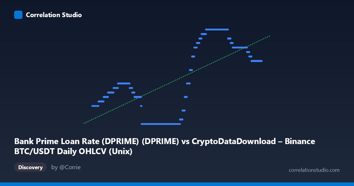
Bank Prime Loan Rate (DPRIME) (DPRIME) vs CryptoDataDownload – Binance BTC/USDT Daily OHLCV (Unix)
- Pearson correlation (r)
- 0.6659
- Spearman correlation
- 0.5801
- p-value
- 0
- Sample size (n)
- 2227
- 95% confidence interval
- 0.6422 to 0.6884
- Granger causality
- None
- Granger optimal lag
- 1
- Time coverage
- 2017-08-17 to 2026-06-25
- Recomputed on refreshed data
- 2026-10-23 (r was 0.6659)
AI analysis
Analysis: Bank Prime Loan Rate vs. BTC/USDT Timestamp
(Note: the axis labels appear swapped in the metadata — X is described as "Bank Prime Loan Rate" but contains Unix timestamps spanning 2017–2026, while Y is described as a timestamp column but contains values in the 3.25–8.50 range, consistent with actual prime rate percentages. This analysis treats X as time and Y as the Bank Prime Loan Rate.)
1. What the Visualization Reveals
The scatterplot shows the trajectory of the U.S. Bank Prime Loan Rate over time (2017–2026), plotted against the corresponding dates of a BTC/USDT price series used as the time index. Rather than showing a relationship between two independent economic phenomena, this chart is essentially a time series of interest rates, with Bitcoin trading dates serving as a proxy timeline. The visual pattern reflects well-known Federal Reserve rate policy: a low, flat rate (~3.25%) during 2020–2021 (near-zero rate era), followed by a steep climb to ~8.5% during 2022–2023 (aggressive tightening cycle), then a plateau/gradual decline into 2024–2026.
2. Strength and Direction of Correlation
The reported r = 0.666 (r² = 0.444) indicates a moderate-to-strong positive relationship, meaning roughly 44% of the variance in the rate is "explained" by the timestamp — but since X is simply time, this really just confirms the rate has a strong upward trend over the sampled window, not a causal or economically meaningful link. The tight 95% CI [0.643, 0.689] and p ≈ 0 reflect high statistical confidence, but with n = 2,221 daily observations that are highly autocorrelated (the rate changes rarely and persists for months), the p-value is misleadingly small — it reflects sample size and serial correlation rather than independent confirmatory evidence. The Granger causality results (p = 0.268 and p = 0.285, both non-significant) confirm there is no meaningful lead-lag predictive relationship here, which makes sense: one variable is literally a time index, so "causality" is not a meaningful concept.
3. Notable Patterns and Non-Linearities
The data is clearly non-linear and regime-based rather than continuous/linear: - A long flat plateau at 3.25% (2020 through mid-2021, and again briefly in 2022) - A sharp step-like ascent through 2022–2023 (3.25% → 8.50%), consistent with 11 consecutive Fed hikes - A high plateau (~8.0–8.5%) through 2023–2024 - A gradual step-down beginning in 2024–2025 toward ~6.75–7.75%
This staircase pattern is a hallmark of policy rates, which move in discrete jumps (25–75 bps) rather than smoothly — a linear regression (R²=0.444) is a poor structural fit despite the moderate correlation coefficient, since a piecewise/step function would capture the data far better.
4. Confounding Factors and Caveats
- Spurious correlation risk: Regressing an interest rate against a timestamp (or against BTC trading dates) conflates two unrelated processes — this is a classic case where correlation reflects shared trend-over-time, not any substantive economic link between Bitcoin and monetary policy. - Autocorrelation inflates significance: Daily prime-rate observations are not independent; the effective sample size is far smaller than n=2,221, making the p-value close to meaningless for hypothesis testing. - Metadata/axis mismatch: The variable descriptions suggest the columns were mislabeled or merged incorrectly, which should be corrected before drawing further conclusions. - Discrete rate changes: The rate only moves ~10–15 times over the entire period, so statistical measures like r² are dominated by a few step-change events, not smooth covariation.
5. Suggested Next Steps
1. Fix the data merge: Confirm which column truly represents which variable — this looks like a join artifact between a BTC OHLCV time series and a FRED rate series using timestamps as keys. 2. Reframe the actual question: If the intent was to study BTC price vs. prime rate (a genuinely interesting macro question), re-run correlation using BTC closing price vs. DPRIME, not the timestamp columns. 2. Use rate regime dummies: Since the prime rate moves in discrete steps, treat rate-hike cycles as categorical regimes and test BTC performance conditional on regime (e.g., hiking vs. cutting periods) rather than raw linear correlation. 3. Test with proper time-series methods: Use cointegration or lagged regression (with BTC returns vs. rate changes) instead of Granger on mismatched series, since the current Granger test is uninformative given the axis error.
X dataset: CryptoDataDownload – Binance BTC/USDT Daily OHLCV
Y dataset: Bank Prime Loan Rate (DPRIME)
Part of experiment: Bitcoin - CryptoDataDownload – Binance BTC/USDT Daily OHLCV vs Bank Prime Loan Rate (DPRIME)