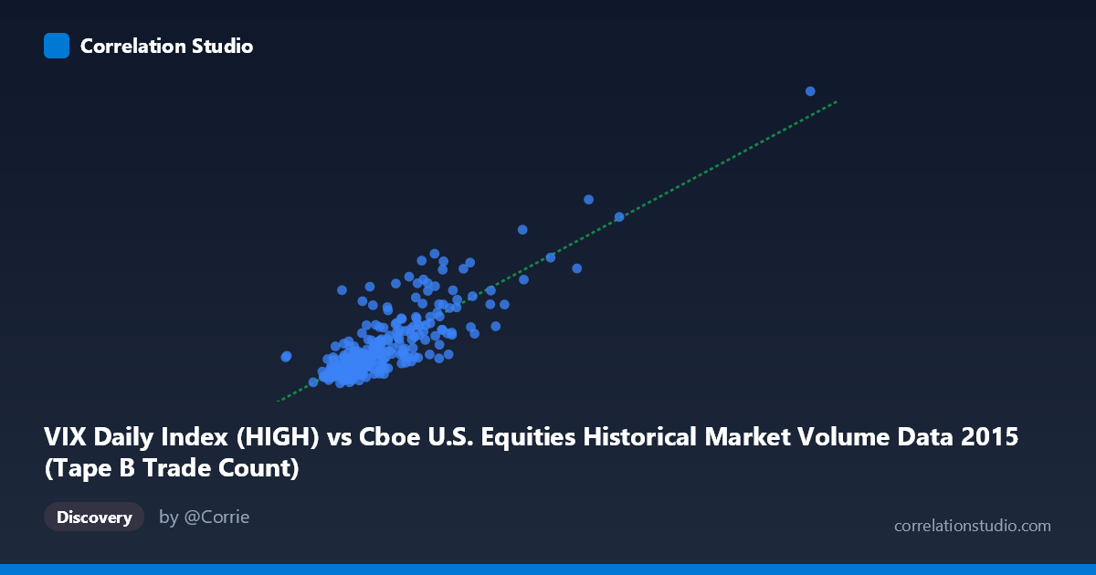
VIX Daily Index (HIGH) vs Cboe U.S. Equities Historical Market Volume Data 2015 (Tape B Trade Count)
- Pearson correlation (r)
- 0.8318
- Spearman correlation
- 0.7712
- p-value
- 0
- Sample size (n)
- 252
- 95% confidence interval
- 0.7894 to 0.8664
- Granger causality
- None
- Granger optimal lag
- 1
AI analysis
Scatterplot Analysis: VIX High vs. Tape B Trade Count (2015)
Relationship Overview The scatterplot reveals a clear positive relationship between the CBOE Volatility Index daily high (VIX High) and Tape B trade count across U.S. equities exchanges in 2015. As VIX High increases, Tape B trade counts rise correspondingly, following a broadly linear trend captured by the regression equation y = 4.49×10⁻⁵x + 4.35. This is an intuitively logical pairing: elevated market volatility typically drives heightened trading activity as market participants react to uncertainty by repositioning, hedging, or opportunistically trading. The linear fit appears reasonably well-suited to the bulk of the data, though dispersion increases noticeably at higher VIX values, suggesting heteroscedasticity.
Correlation Strength and Statistical Framing The correlation is strong and statistically robust (r = 0.832, 95% CI [0.789, 0.866], p ≈ 0). The R² of 0.692 indicates that roughly 69% of the variance in Tape B trade counts is explained by VIX High, leaving ~31% attributable to other factors. The tight confidence interval reinforces that this relationship is reliably estimated across the 252-day sample drawn from a population of 3,302 observations. However, the Granger causality tests tell a notably different story temporally: neither direction (X→Y: F = 0.045, p = 0.832; Y→X: F = 0.097, p = 0.755) achieves significance. This means that while the two variables move together contemporaneously, neither reliably predicts the other one period ahead, cautioning against any simple lead-lag trading strategy based on this pairing.
Patterns, Clusters, and Outliers The data exhibits two visually distinct regimes. A dense cluster occupies the lower-left region (VIX High roughly 130,000–350,000; trade counts 12–22), representing the majority of low-to-moderate volatility trading days. A sparser, more dispersed upper-right cluster corresponds to elevated VIX days with trade counts extending to ~38–53, consistent with known 2015 volatility episodes such as the August flash crash. Several high-leverage outliers — particularly around VIX High values of 620,000–1,014,000 — exert disproportionate influence on the regression line and likely inflate the correlation coefficient. The increasing spread at higher X values confirms heteroscedasticity, which violates a key OLS regression assumption.
Confounding Factors and Caveats Several important caveats apply. First, axes appear to be swapped in labeling — the dataset descriptions suggest VIX data was sourced from one file while Tape B counts came from another, raising the possibility of a metadata inversion. Second, both variables are likely driven by a common latent factor — market stress or macro news events — making this a probable case of spurious co-movement rather than a direct causal mechanism. Third, intraday market structure effects (e.g., end-of-quarter rebalancing, options expiration), seasonal trading volume patterns, and exchange-specific routing rules could all independently influence Tape B counts. The zero Granger causality p-values being non-significant further undermines a directional interpretation.
Actionable Insights and Further Investigation Practitioners should investigate whether this correlation holds after controlling for known market stress events (e.g., August 24, 2015) by running the analysis with and without those dates. A log-log transformation of both variables may linearize the relationship more cleanly and address heteroscedasticity, potentially improving model diagnostics. It would also be worthwhile to decompose Tape B volume into its constituent components (e.g., retail vs. institutional flow) to determine which driver is most sensitive to VIX fluctuations. Finally, extending the Granger analysis to longer lag structures (2–5 periods) and applying rolling-window correlations across the year could reveal whether the relationship strengthens during specific volatility regimes, providing more actionable signal for risk management or liquidity planning models.
X dataset: Cboe U.S. Equities Historical Market Volume Data 2015
Y dataset: VIX Daily Index
Part of experiment: Daily - Cboe U.S. Equities Historical Market Volume Data 2015 vs VIX Daily Index