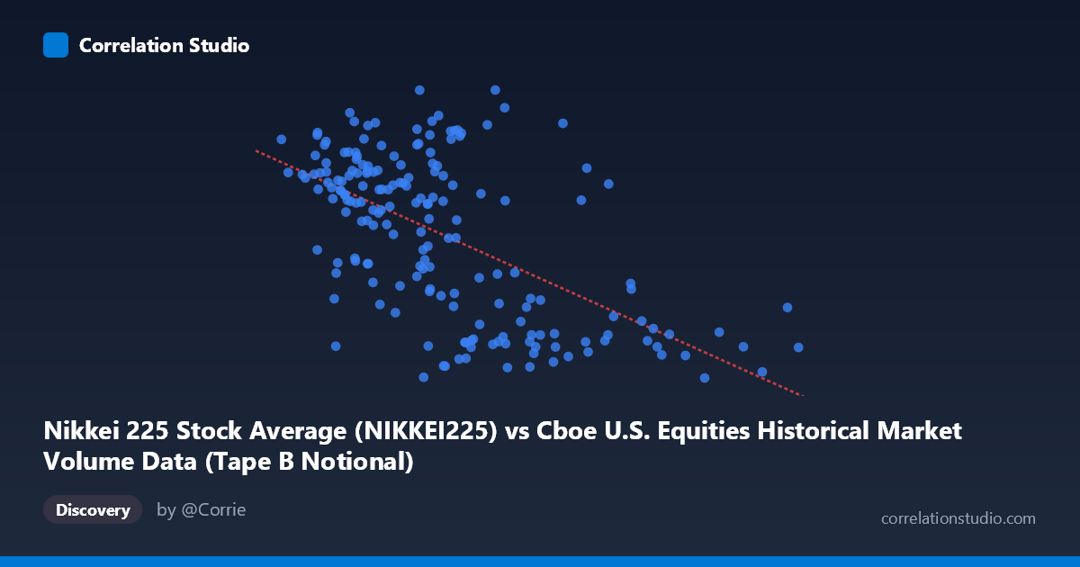
Nikkei 225 Stock Average (NIKKEI225) vs Cboe U.S. Equities Historical Market Volume Data (Tape B Notional)
- Pearson correlation (r)
- -0.5888
- Spearman correlation
- -0.5383
- p-value
- 0
- Sample size (n)
- 187
- 95% confidence interval
- -0.6753 to -0.4864
- Granger causality
- None
- Granger optimal lag
- 10
- Time coverage
- 2026-01-05 to 2026-10-21
- Recomputed on refreshed data
- 2026-10-23 (r was -0.5888)
AI analysis
Scatterplot Analysis: Nikkei 225 vs. Cboe Tape B Notional Volume
Relationship Overview
The scatterplot reveals a moderate negative relationship between the Nikkei 225 index level and Cboe U.S. Equities Tape B Notional Volume over the January–May 2026 period. As Nikkei 225 values increase (roughly 7.1B to 21.0B on the x-axis, reflecting index-level scaling), Tape B notional volume tends to decline. The linear regression equation (y = -5.99993E-07x + 63,655) captures this downward slope visually, with the data cloud tilting from upper-left to lower-right. However, the scatter around the regression line is substantial, indicating this relationship is real but far from deterministic — many individual days deviate considerably from the trend.
Correlation Strength and Statistical Significance
The Pearson correlation of r = -0.569 indicates a moderate negative association, and the R² of 0.324 means that approximately 32.4% of the variance in Tape B notional volume is statistically explained by the Nikkei 225 level — leaving roughly 67.6% of variance unexplained by this relationship alone. The 95% confidence interval for r spans [-0.694, -0.410], which is meaningfully wide but does not cross zero, reinforcing that the direction of the relationship is reliable. The p-value of 4.88 × 10⁻⁹ is highly significant given the sample of n = 90, making it extremely unlikely this correlation arose by chance. That said, Granger causality tests reveal no significant temporal predictive direction in either direction (X→Y: F = 1.66, p = 0.112; Y→X: F = 1.27, p = 0.269), meaning neither variable reliably predicts the other's future values at the tested lags. This is a critical caveat: the correlation is contemporaneous and structural, not predictive in a causal time-series sense.
Notable Patterns, Clusters, and Outliers
Several features stand out in the data. There is a visible cluster of high Tape B volume observations (≥60,000) concentrated in the lower Nikkei range (~7.6B–11.0B), suggesting elevated U.S. equity activity coincides with periods of lower Japanese market levels. Conversely, observations in the upper Nikkei range (≥17B) almost uniformly show lower Tape B notional values (≤55,000), forming a relatively tight cluster. A few potential outliers merit attention: the point near (20,657B, 56,279) sits notably above the regression line for its Nikkei level, and (10,174B, 51,117) and (10,792B, 51,940) show unusually low Tape B volume for their Nikkei position, pulling against the general trend. The relationship also appears somewhat non-linear — the decline in Tape B volume appears steeper at lower Nikkei levels and flattens as Nikkei rises, hinting that a logarithmic or segmented fit might capture the data better than the linear model.
Confounding Factors and Interpretation Caveats
The most important caveat here is the dataset labeling asymmetry — the X-axis draws Nikkei 225 data from what is labeled a Cboe dataset, and the Y-axis draws Tape B notional data from what is labeled a Nikkei dataset. This cross-labeling strongly suggests a data alignment or metadata mismatch that warrants verification before drawing any substantive conclusions. Beyond that, several genuine confounders could drive the observed correlation: global risk-off/risk-on regimes could simultaneously suppress Japanese equities and spike U.S. trading volumes; currency movements (USD/JPY) influence both markets; macro events (FOMC decisions, geopolitical shocks) during this short five-month window could create spurious co-movement; and seasonal or calendar effects (e.g., Japanese fiscal year-end in March) may introduce systematic patterns unrelated to any direct link between the two variables.
Actionable Insights and Further Investigation
Given the moderate but statistically robust correlation and the absence of Granger causality, the most productive next steps would be: (1) Verify data provenance — confirm that the Nikkei and Tape B columns are correctly matched to their respective datasets and that the index values on the x-axis (7.1B–21.0B range, which is atypically scaled for Nikkei) represent the correct units; (2) Introduce control variables such as VIX (volatility index), USD/JPY exchange rates, and S&P 500 levels to partial out common global drivers; (3) Test non-linear models (e.g., logarithmic regression or piecewise linear) given the visual evidence of a flattening relationship at higher Nikkei levels; (4) Extend the time series beyond five months — with N = 1,980 total observations available, using the full dataset would substantially sharpen confidence intervals and enable more robust Granger causality testing at multiple lags; and (5) Examine lagged cross-correlations at shorter intervals (1–5 days) since the optimal lag of 10 periods in Granger testing may be masking shorter-horizon predictive signals.
X dataset: Cboe U.S. Equities Historical Market Volume Data
Y dataset: Nikkei 225 Stock Average
Part of experiment: Daily - Cboe U.S. Equities Historical Market Volume Data vs Nikkei 225 Stock Average