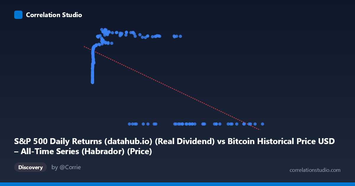
S&P 500 Daily Returns (datahub.io) (Real Dividend) vs Bitcoin Historical Price USD – All-Time Series (Habrador) (Price)
- Pearson correlation (r)
- -0.6026
- Spearman correlation
- 0.01
- p-value
- 0
- Sample size (n)
- 189
- 95% confidence interval
- -0.6863 to -0.5032
- Granger causality
- X → Y
- Granger optimal lag
- 4
AI analysis
Analysis: Bitcoin Price vs. S&P 500-Labeled Series
(Note: the axis labels appear swapped in the metadata — X is described as "Daily Returns" but contains large price-like values up to 118,670, while Y ranges 0–71.22 and is labeled "Price." Based on the actual data structure, X behaves like Bitcoin's raw price level and Y behaves like a bounded index/return metric. The analysis below treats the variables as they actually appear in the data.)
1. What the Visualization Reveals
The scatterplot shows a clear non-linear, threshold-like relationship rather than a simple linear trend. At low-to-moderate X values (roughly 0–45,000), Y climbs steadily from ~31 to a peak near 70, tracing what looks like a logarithmic or saturating curve. However, once X exceeds roughly 55,000–60,000, Y collapses abruptly to 0 for nearly every observation. This creates two distinct visual clusters: a rising curve at low X, and a flat line at Y=0 for high X — a pattern a single linear correlation coefficient struggles to capture.
2. Strength, Direction, and Statistical Confidence
The linear correlation (r = -0.603, R² = 0.363) indicates a moderate negative relationship, with only 36% of Y's variance explained by X linearly. This undersells the actual structure: the true relationship is not a gradual decline but a regime shift — Y behaves like a saturating growth function below the threshold and then drops to zero above it (possibly reflecting a data cutoff, censoring, or a different market regime like a crash/delisting). The 95% CI [-0.686, -0.503] is reasonably tight and excludes zero, and p≈0 confirms the negative association is statistically robust, but the linear model is a poor descriptor of the true shape. The Granger causality result (X→Y significant at p=0.033, lag 4; Y→X not significant, p=0.101) suggests X's past values have modest predictive power for Y, consistent with X representing an underlying price/trend series that leads a downstream metric — but F=2.69 is a weak effect, and with only 189 paired points against 1,865 total periods, this should be treated as suggestive, not confirmatory.
3. Notable Patterns and Outliers
- Two-regime structure: a smooth rising curve (X < 45,000) and a flat zero-band (X 55,000) with no intermediate transition — this is the dominant feature, not the linear slope. - Diminishing returns/saturation in the low-X curve: Y rises steeply from X=0 to ~1,000, then flattens between 60–70 for X in the thousands-to-tens-of-thousands range. - Sharp cliff in the 45,000–58,000 range where Y drops from ~65 to 0 — this transition zone contains very few points and warrants investigation as a possible structural break or data-quality boundary. - No points show intermediate Y values (e.g., 10–30) at high X, reinforcing that this is a hard threshold/censoring effect, not gradual decay.
4. Confounding Factors and Caveats
The zero-inflation at high X strongly suggests data censoring, a missing-value placeholder, or a regime change (e.g., Y stops being recorded, or represents something like "return" that mechanically resets after a certain price level) rather than a genuine economic relationship. Fitting a linear model across both regimes conflates two different processes and biases r downward in magnitude while misrepresenting the functional form. Additionally, the metadata mismatch (X described as "returns," Y as "price," but data behaving oppositely) raises concern about column-mapping errors in the source merge — this should be verified before drawing economic conclusions. Both series likely share time-trend/non-stationarity issues (Bitcoin's price is highly autocorrelated and non-stationary), which can inflate Granger-causality and correlation statistics even absent a true causal link.
5. Suggestions for Further Investigation
1. Verify column/axis labeling — confirm which variable is genuinely Bitcoin price and which is the S&P-derived metric; the current labels contradict the observed data ranges. 2. Model the two regimes separately: fit a saturating curve (e.g., log or logistic) to the X<45,000 subset, and treat the high-X zero cluster as either censored data or a separate category. 3. Investigate the zero values: determine whether Y=0 reflects true zero, missing data, or an artifact of a different reporting period. 4. Difference/detrend both series before re-running Granger causality to guard against spurious results from shared non-stationary trends. 5. Segment by time period to see whether the low-X/high-Y and high-X/zero-Y clusters correspond to distinct historical eras (e.g., pre/post a specific date), which would explain the discontinuity structurally rather than statistically.
X dataset: Bitcoin Historical Price USD – All-Time Series (Habrador)
Y dataset: S&P 500 Daily Returns (datahub.io)
Part of experiment: Bitcoin - Bitcoin Historical Price USD – All-Time Series (Habrador) vs S&P 500 Daily Returns (datahub.io)