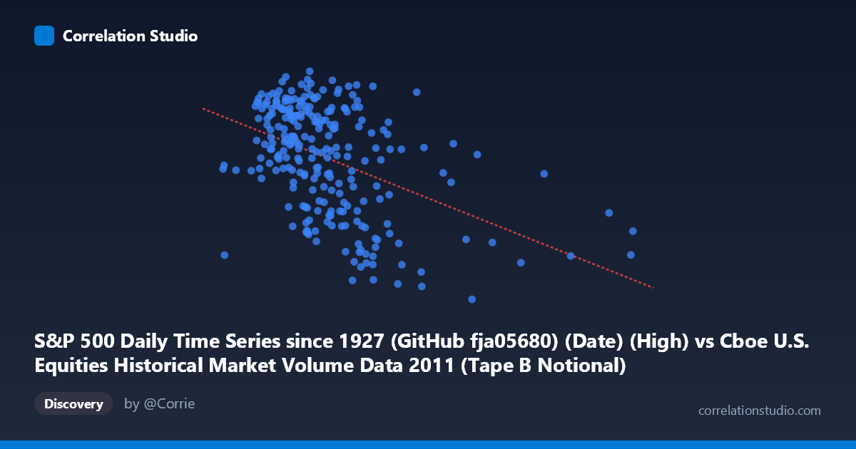
S&P 500 Daily Time Series since 1927 (GitHub fja05680) (Date) (High) vs Cboe U.S. Equities Historical Market Volume Data 2011 (Tape B Notional)
- Pearson correlation (r)
- -0.4508
- Spearman correlation
- -0.4296
- p-value
- 0
- Sample size (n)
- 252
- 95% confidence interval
- -0.5441 to -0.3466
- Granger causality
- None
- Granger optimal lag
- 1
AI analysis
Analysis: S&P 500 High vs. Cboe Tape B Notional Value (2011)
Relationship Overview The scatterplot reveals a moderate negative relationship between the S&P 500 daily high price (X-axis) and Cboe Tape B notional trading value (Y-axis) across 252 trading days in 2011. As the S&P 500 index level rises, Tape B notional value tends to decline, and vice versa. This inverse pattern is visually apparent as a downward-sloping cloud of points, with higher index values (roughly above 7–8 billion on the x-axis) clustering toward lower Tape B notional values, while lower index readings concentrate around higher notional figures. The linear regression equation (y = -1.46×10⁻⁸x + 1351.92) quantifies this slope, suggesting each unit increase in the S&P 500 high corresponds to a modest but consistent decrease in Tape B notional value.
Correlation Strength and Statistical Significance The Pearson correlation of r = -0.4508 indicates a moderate negative association. However, the coefficient of determination r² = 0.2033 is the more practically meaningful figure — it tells us that only ~20.3% of the variance in Tape B notional value is statistically explained by the S&P 500 high. The remaining ~80% of variation is driven by factors outside this simple linear model. The 95% confidence interval of [-0.5441, -0.3466] is meaningfully negative throughout, excluding zero entirely, and the p-value of 5.09×10⁻¹⁴ confirms this correlation is extraordinarily unlikely to arise by chance, even with N=3,780 population points. That said, statistical significance here is partly a function of large sample size — the effect, while real, is not large. Importantly, Granger causality tests show no significant temporal predictive direction in either direction (X→Y: F=0.13, p=0.72; Y→X: F=0.07, p=0.79), meaning that knowing today's S&P 500 high does not help predict tomorrow's Tape B notional, and vice versa. The correlation reflects a contemporaneous association, not a leading/lagging predictive relationship.
Notable Patterns, Clusters, and Outliers The data cloud shows a broadly scattered distribution with a discernible but noisy downward trend. Several features stand out. First, there is a visible cluster of high-activity points in the x-range of roughly 3.0–5.5 billion, where Tape B notional values span widely from ~1,160 to ~1,370, suggesting high within-cluster variability that weakens the linear fit. Second, there are notable outliers at the high end of the x-axis — points around 9.5–14 billion in the S&P 500 high — that consistently sit at lower Tape B notional values (~1,150–1,290), pulling the regression line downward. Third, the Y-axis range is relatively compressed (1,125–1,371, a span of ~245 units), which visually amplifies scatter. The relationship appears weakest in the mid-range of X, consistent with higher residual variance there.
Confounding Factors and Interpretive Caveats Several important caveats apply. The axis labels appear swapped in interpretation: the X-axis is labeled as "Date (High)" from the S&P 500 dataset while the Y-axis references "Tape B Notional" from a Cboe dataset — it's worth verifying the join key used (likely date-based) is correctly aligned. More substantively, 2011 was a highly unusual market year, marked by the U.S. debt ceiling crisis (August 2011), S&P's U.S. credit downgrade, and significant European sovereign debt volatility — these episodic stress events likely drive much of the observed pattern, as market dislocations simultaneously suppress index levels and spike volume/notional activity. Tape B specifically covers NYSE American and regional exchange stocks, not the broad market, so its notional value reflects segment-specific dynamics. Additionally, secular trends within 2011 (the market fell sharply in August–September and partially recovered) could create spurious correlation through shared time-trend, a classic confound in financial time series.
Actionable Insights and Further Investigation Given the moderate correlation and absent Granger causality, practitioners should not use S&P 500 price levels as a predictive signal for Tape B notional flow. Instead, this relationship is better understood as a contemporaneous, regime-driven phenomenon. Recommended next steps include: (1) segmenting the data by market regime (pre/post August 2011 stress event) to test whether the correlation holds in calm vs. volatile periods; (2) testing non-linear specifications (e.g., polynomial or piecewise regression) given the apparent heteroscedasticity in the mid-x range; (3) including VIX as a covariate, since volatility likely mediates both index level and notional trading activity simultaneously; (4) expanding to Tape A and Tape C notional values to assess whether this inverse pattern is consistent across exchange segments; and (5) repeating the Granger test at longer lags (2–5 periods) to rule out slower predictive dynamics not captured at lag-1.
X dataset: Cboe U.S. Equities Historical Market Volume Data 2011
Y dataset: S&P 500 Daily Time Series since 1927 (GitHub fja05680) (Date)
Part of experiment: Daily - Cboe U.S. Equities Historical Market Volume Data 2011 vs S&P 500 Daily Time Series since 1927 (GitHub fja05680) (Date)