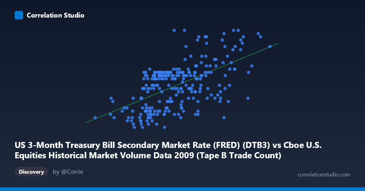
US 3-Month Treasury Bill Secondary Market Rate (FRED) (DTB3) vs Cboe U.S. Equities Historical Market Volume Data 2009 (Tape B Trade Count)
- Pearson correlation (r)
- 0.5768
- Spearman correlation
- 0.5624
- p-value
- 0
- Sample size (n)
- 250
- 95% confidence interval
- 0.4876 to 0.6541
- Granger causality
- None
- Granger optimal lag
- 1
AI analysis
Analysis: US 3-Month T-Bill Rate vs. Cboe Tape B Trade Count (2009)
Relationship Overview The scatterplot reveals a moderate positive relationship between the US 3-Month Treasury Bill Secondary Market Rate and Cboe Tape B equity trade counts during 2009. As T-bill rates increase, trade counts tend to rise as well, though with considerable scatter around the trend line. The linear regression equation (y = 3.25×10⁻⁷x + 0.019421) confirms this positive slope, meaning higher T-bill rates are associated with greater trading activity in Tape B equities. This relationship is visually coherent but far from deterministic, with substantial dispersion across the full range of both variables.
Correlation Strength and Statistical Significance The correlation coefficient of r = 0.5768 indicates a moderate positive association, but the more telling statistic is r² = 0.3327 — meaning only 33.3% of the variance in Tape B trade counts is explained by T-bill rates. Nearly two-thirds of the variation remains attributable to other factors. The 95% confidence interval of [0.4876, 0.6541] is reasonably tight and does not cross zero, and the p-value of effectively 0 across n = 250 paired observations (from a population of N = 3,232) confirms this is not a chance association. However, the Granger causality results complicate any causal interpretation: neither direction (X→Y: F = 1.36, p = 0.24; Y→X: F = 0.55, p = 0.46) achieves statistical significance at conventional thresholds. This means that, at a 1-period lag, neither variable temporally predicts the other, suggesting the observed correlation reflects co-movement driven by a shared underlying factor rather than a direct predictive relationship.
Patterns, Clusters, and Outliers The data exhibits a notable bimodal or clustered structure. A dense cluster of points sits in the lower-left region (T-bill rates approximately 81,000–350,000; trade counts 0.02–0.12), while a second cluster occupies the upper-right (rates 450,000–766,000; trade counts 0.18–0.32). This clustering suggests the relationship may not be smoothly linear but rather reflective of two distinct market regimes during 2009 — consistent with the dramatic volatility of the post-financial-crisis recovery period. Several outliers are visible, including the extreme right-side point near (766,763, 0.27) and a high-trade-count point at (624,611, 0.32), while low-rate observations like (81,703, 0.05) and (231,712, 0.03) anchor the lower-left. The spread widens at higher X values, suggesting possible heteroscedasticity.
Confounding Factors and Caveats Several important caveats apply. First, 2009 was an extraordinary year marked by the tail end of the global financial crisis, stimulus interventions, and extreme market volatility — conditions that simultaneously suppressed T-bill rates early in the year and disrupted normal trading patterns. The apparent correlation may largely reflect a shared time trend: both variables were evolving throughout 2009 in response to the same macroeconomic forces (Fed policy, market stabilization) rather than influencing each other directly. The lack of Granger causality supports this interpretation. Additionally, the axes appear to represent very different scales and units, and the dataset labels suggest a possible axis inversion in the metadata (each dataset's description appears attached to the opposite axis label), which warrants verification before drawing firm conclusions.
Actionable Insights and Further Investigation Given the absence of Granger causality, researchers should resist interpreting this as a predictive relationship and instead investigate common drivers — particularly Fed policy signals, VIX levels, or broader market liquidity conditions — that may explain both variables simultaneously. A time-series decomposition to remove the shared 2009 trend would test whether the correlation persists after detrending. Extending the analysis to multiple years would determine if 2009's crisis context is driving the result. Regime-switching models or segmented regression could formally test whether the apparent two-cluster structure reflects genuinely distinct market states. Finally, confirming the correct axis assignments and variable definitions is essential before publishing or acting on these findings.
X dataset: Cboe U.S. Equities Historical Market Volume Data 2009
Y dataset: US 3-Month Treasury Bill Secondary Market Rate (FRED)
Part of experiment: Daily - Cboe U.S. Equities Historical Market Volume Data 2009 vs US 3-Month Treasury Bill Secondary Market Rate (FRED)