WTI and Brent Oil Prices Dataset (cpi_index) vs Brent Crude Oil Prices: Daily (DCOILBRENTEU) – FRED St. Louis Fed (DCOILBRENTEU)
- Pearson correlation (r)
- 0.7331
- Spearman correlation
- 0.7807
- p-value
- 0
- Sample size (n)
- 295
- 95% confidence interval
- 0.6754 to 0.7818
- Granger causality
- None
- Granger optimal lag
- 4
AI analysis
Analysis: CPI-Adjusted WTI vs. Nominal Brent Crude Oil Prices
Relationship Overview
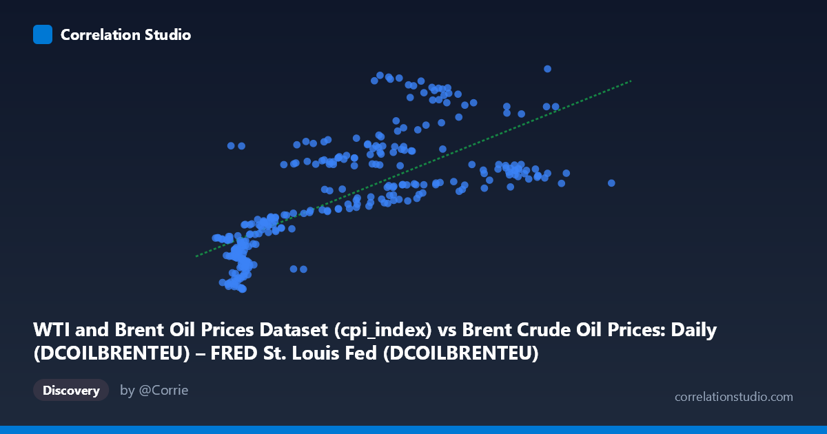
The scatterplot reveals a moderately strong positive relationship between nominal Brent crude oil prices (X) and CPI-adjusted WTI crude prices (Y), with the linear regression equation y = 1.212x + 142.03 describing the central tendency. As nominal Brent prices rise, real WTI prices rise correspondingly — an expected finding given that these are two measures of closely related crude oil benchmarks. However, the scatter around the regression line is notably wide, particularly in the mid-to-upper range of X values (roughly 50–120 USD/barrel), where Y values span nearly 200 points (approximately 130–330), suggesting that the two series diverge meaningfully during specific market episodes despite their general co-movement.
Correlation Strength and Statistical Framing
The Pearson correlation of r = 0.733 (95% CI: [0.675, 0.782], p ≈ 0) confirms a statistically robust positive association across the 295 paired observations spanning 1987–2026. The R² = 0.537 is the more practically important figure: nominal Brent prices explain only about 54% of the variance in real WTI prices, meaning roughly 46% of variation remains unaccounted for by this simple linear model. The confidence interval is relatively tight, ruling out a weak relationship, but the upper bound of 0.782 still falls short of the near-unity correlation one might naively expect between two crude benchmarks. Importantly, Granger causality tests show no statistically significant predictive direction in either direction (X→Y: F = 1.23, p = 0.300; Y→X: F = 1.62, p = 0.169), even at the optimal lag of 4 periods. This means that past values of nominal Brent do not significantly help predict future real WTI values beyond what is already captured in real WTI's own history, and vice versa — a notable finding that tempers any causal narrative between these series.
Notable Patterns, Clusters, and Outliers
The sample data reveals a pronounced bimodal clustering structure. A dense cluster of low-price observations occupies the region X < 30, Y < 180, corresponding to the pre-2000s era of depressed oil prices. A second, more diffuse cloud spans X = 50–130, Y = 180–330, reflecting the post-2000 commodity supercycle and COVID-era volatility. Several high-leverage outliers stand out: the points at approximately (62.37, 320.62) and (75.30, 315.63) show unusually high real WTI values relative to their Brent levels, likely reflecting specific inflationary adjustment periods or WTI-Brent spread anomalies (such as the 2011–2013 WTI discount driven by Cushing, Oklahoma storage bottlenecks). Conversely, some high-Brent observations (X 100) yield only moderate real WTI values (~230), suggesting CPI deflation erodes the apparent price spike. The relationship also appears to exhibit mild non-linearity or heteroscedasticity, with variance in Y increasing as X increases.
Confounding Factors and Caveats
Several important caveats apply. First, this analysis conflates two conceptually distinct variables: nominal Brent (a raw price) versus real CPI-adjusted WTI (an inflation-corrected price for a different — though highly correlated — benchmark). The correlation partially reflects the mechanical relationship between nominal and real prices rather than independent market dynamics. Second, CPI adjustment methodology introduces a constructed variable component; the choice of CPI deflator, base year, and revision vintage all affect the real series. Third, the 1987–2026 time window spans multiple structurally different oil market regimes — OPEC quota systems, the shale revolution, COVID demand collapse, and geopolitical supply shocks — meaning the linear model may mask regime-specific sub-relationships. Finally, the large gap between the two clusters may create spurious statistical inflation of the correlation coefficient that wouldn't hold within each sub-period independently.
Actionable Insights and Further Investigation
Practitioners should avoid treating this correlation as a reliable real-time forecasting tool, given the failed Granger causality tests and the 46% unexplained variance. Instead, several follow-up analyses are warranted: (1) Segment the data by market regime (pre-2000, 2000–2014 supercycle, post-shale, post-COVID) and compute regime-specific correlations to test whether the relationship is stable or structural; (2) model the WTI-Brent spread explicitly as the dependent variable, using inflation, pipeline capacity, and geopolitical risk indices as predictors; (3) apply cointegration testing (e.g., Engle-Granger or Johansen) to determine whether these series share a long-run equilibrium relationship despite the absence of Granger causality at short lags; (4) consider a non-linear or piecewise regression to better capture the heteroscedastic fan structure visible in the mid-range. The dataset's length (nearly 40 years) provides excellent statistical power for such sub-analyses.
X dataset: Brent Crude Oil Prices: Daily (DCOILBRENTEU) – FRED St. Louis Fed
Y dataset: WTI and Brent Oil Prices Dataset
Part of experiment: Daily - Brent Crude Oil Prices: Daily (DCOILBRENTEU) – FRED St. Louis Fed vs WTI and Brent Oil Prices Dataset